Fine-Tuning EfficientNetB0 for Bird Species Image Classification
Transfer learning is a machine learning technique that reuses patterns learned by a pre-trained model on a new dataset and task. In my previous post “TensorFlow: Transfer Learning (Feature Extraction) in Image Classification”, I wrote about employing pre-trained models such as EfficientNet — trained on the ImageNet dataset and available in the TensorFlow Hub — for the task of bird species prediction. That earlier post covered the feature extraction approach. This post applies the fine-tuning approach I learned in the Udemy course on TensorFlow, describing transfer learning experiments that fine-tune a bird species prediction model. The code uses the Keras EfficientNet API for building EfficientNetB0-based models.
What Is Fine-Tuning in Transfer Learning?
Fine-tuning is a transfer learning method that unfreezes some layers of a pre-trained model and retrains them at a low learning rate to adapt learned features to a new dataset. In transfer learning, we reuse features learned on a different dataset for a different problem — useful when training data is limited and a state-of-the-art, well-tested model such as EfficientNet [5] is available. Transfer learning thus reuses features extracted from an existing model for predictions on a new dataset.
Figure 1 schematically shows the difference between feature extraction (see my post on feature extraction) and fine-tuning in transfer learning. I have drawn it to outline the process of using the trained on ImageNet model, in which layers are frozen during the feature extraction step. After the model is converged with the use of the birds’ dataset, we unfreeze some unfrozen layers while performing fine-tuning wherein the model is retrained with new data using the bird species dataset [2].
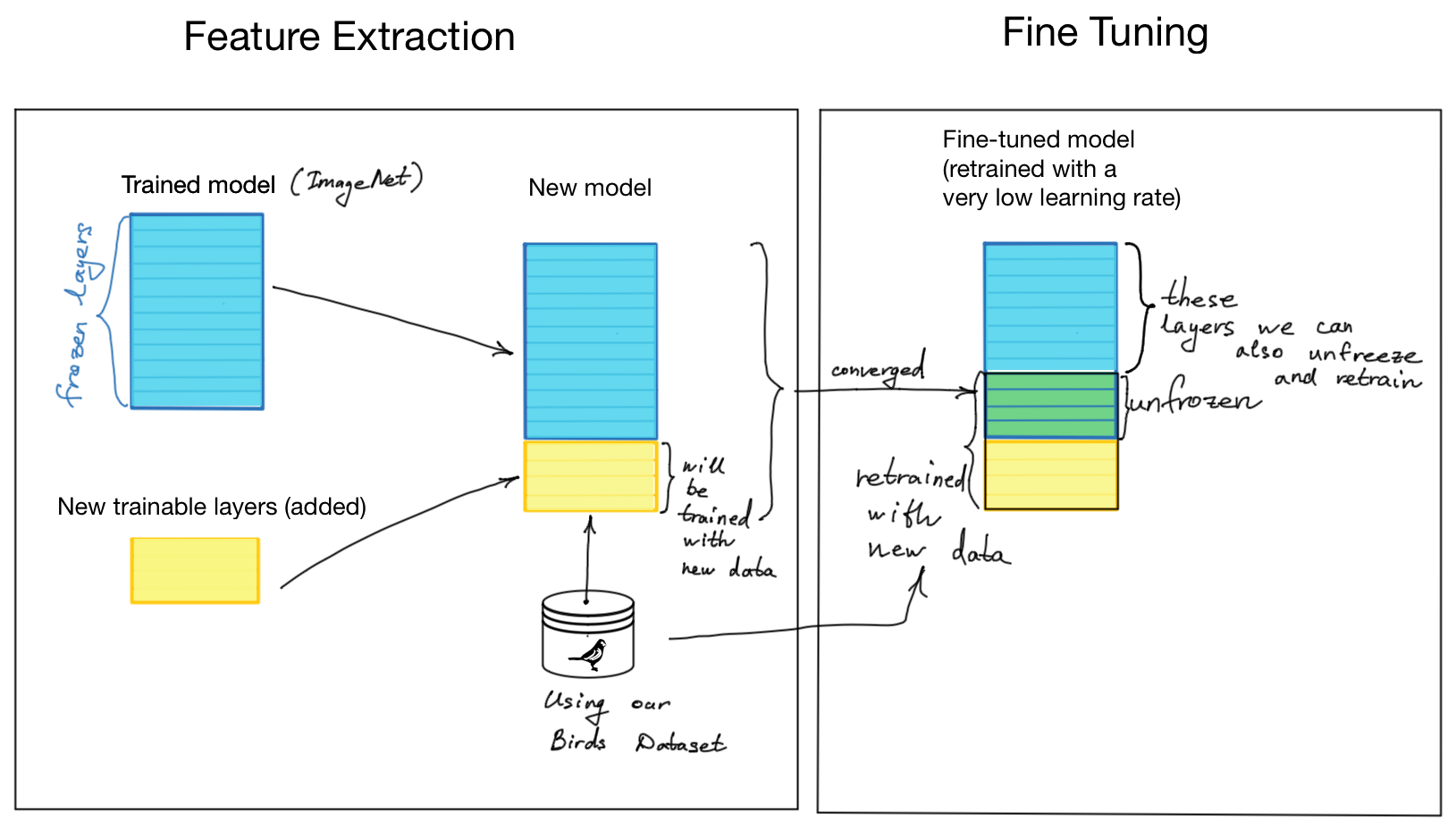
Figure 1. Transfer Learning: feature extraction vs fine-tuning
The fine-tuning is done by unfreezing the frozen layers, partially or entirely, and retraining the model with a meager learning rate. This way, we adapt the trained features to our new (birds species) dataset while (potentially) achieving better prediction results.
Would fine-tuning be beneficial to our bird species prediction task? Let’s run some experiments on feature extraction with fine-tuning and comparing their results with the feature extraction without fine-tuning (the model described and evaluated in my previous post on feature extraction).
Retrieving and Preparing the 400 Bird Species Dataset
I have described the data loading and preprocessing in my previous post
“TensorFlow: Transfer Learning (Feature Extraction) in Image Classification”
in detail. You could read it if you did not do it yet. I also moved the code that
I will further reuse it in the GiHub repository, helpers.py.
You can check it out and use it for your own convenience.
This code is adapted from the Udemy course
and includes getting and unzipping the dataset, preprocessing, plotting images, and loss
functions, model creation and callbacks for TensorBoard and saving of checkpoints
for deep learning experiments with TensorFlow.
You can use this code directly in Colab with:
!wget https://raw.githubusercontent.com/edaehn/deep_learning_notebooks/main/helpers.py
Downloading the Kaggle Bird Species Dataset with kaggle.json
I will reuse the code from my previous post (you can download the code from my repository). Since we will compare our final model performance with the model’s performance without fine-tuning with augmented data, we will also augment data. This should give a meaningful comparison and help reduce overfitting. With the code, we retrieve and augment the 400 Bird Species Dataset [2]. Please note that you need to generate your “kaggle.json” file for retrieving this dataset from Kaggle website.
# Setup to download Kaggle datasets into a Colab instance
! pip install kaggle
! mkdir ~/.kaggle
! cp kaggle.json ~/.kaggle/
! chmod 600 ~/.kaggle/kaggle.json
! kaggle datasets download gpiosenka/100-bird-species/birds -p /content/sample_data/birds --unzip
With the walk_directory() function in helpers.py we check how many images are stored in the “train,” “valid,” “test” and “images to test” directories. All three directories contain 400 directories named bird species, in which there are at least five bird images. We have only five bird images in train and valid (for validation) datasets. In comparison, we have at least a hundred bird images in the training dataset. We have seven bird images in the “images to test” directory.
# Import all functions from the helpers.py
from helpers import *

# Define the directory wherein the dataset is stored
dataset_path = "sample_data/birds"

# Show file numbers in the directory "sample_data/birds"
walk_directory(dataset_path)
There are 4 directories and '5'' files in sample_data/birds.
There are 400 directories and '0'' files in sample_data/birds/train.
There are 0 directories and '127'' files in sample_data/birds/train/ROUGH LEG BUZZARD.
There are 0 directories and '137'' files in sample_data/birds/train/BLACK-NECKED GREBE.
...
There are 400 directories and '0'' files in sample_data/birds/valid.
There are 0 directories and '5'' files in sample_data/birds/valid/ROUGH LEG BUZZARD.
There are 0 directories and '5'' files in sample_data/birds/valid/BLACK-NECKED GREBE.
There are 0 directories and '5'' files in sample_data/birds/valid/WHITE BROWED CRAKE.
...
There are 400 directories and '0'' files in sample_data/birds/test.
There are 0 directories and '5'' files in sample_data/birds/test/ROUGH LEG BUZZARD.
There are 0 directories and '5'' files in sample_data/birds/test/BLACK-NECKED GREBE.
There are 0 directories and '5'' files in sample_data/birds/test/WHITE BROWED CRAKE.
...
There are 0 directories and '7'' files in sample_data/birds/images to test.
Let’s see five random birds with show_five_birds() function to see that the dataset is well unpacked.
show_five_birds()
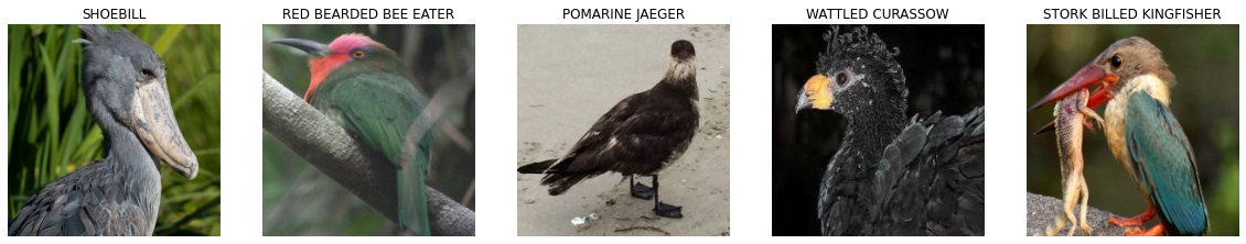
Figure 2. Five Random Birds from the Training Dataset
Loading the Dataset with image_dataset_from_directory()
In Keras preprocessing module, we have the image_dataset_from_directory() function making it easy to load datasets from disk.
# Defining train and test directories
train_directory = dataset_path + "/train"
test_directory = dataset_path + "/test"

# Setup data inputs
IMG_SIZE = (224, 224)
train_data = tf.keras.preprocessing.image_dataset_from_directory(
    train_directory,
    label_mode="categorical",
    image_size=IMG_SIZE
)

test_data = tf.keras.preprocessing.image_dataset_from_directory(
    test_directory,
    label_mode="categorical",
    image_size=IMG_SIZE,
    shuffle=False
)
Found 58388 files belonging to 400 classes.
Found 2000 files belonging to 400 classes.
Preprocessing the Dataset with a Data Augmentation Layer
In the previous post adopting the Udemy course code, we used the preprocess_and_augment_data() function that performs data augmentation to minimise model overfitting, which is quite important when we have complex models and a relatively small dataset, as in our case. Herein, we add data augmentation as a layer using the Sequential model.
Model Creation: Four EfficientNetB0 Transfer Learning Variants
Next, we are going to create and compare three models:
- Baseline model build on top of EfficientNetB0 (see Keras API) and trained with ImageNet data. We add an output layer with 400 Bird Species classes. We add a few layers for converging the model with the new data we want to use.
- Baseline model the same as (1) using augmented dataset.
- A fine-tuned version of the baseline model also uses augmented data (2), retrained at a meager learning rate.
- A final model is created on the insights we got from the evaluation results of our previous models.
Saving Model Checkpoints with ModelCheckpoint Callbacks
When running our experiments, model training can take loads of time. This process can sometimes be interrupted. We might also want to continue model training later. This is why it is useful to continuously save model weights during the training. We create CheckPoint callbacks that save model weights at each epoch of training (when we have defined save_freq=”epoch”). Later, we can load the model weights stored in the checkpoint files and use the model in predictions or in the evaluation process. I have included the create_checkpoint_callback() function into the helpers.py file.
# Creating checkpoint callbacks for usage in model.fit()
def create_checkpoint_callback(checkpoint_path=\
          "tmp/birds_model_3_fine_tuned/checkpoint.ckpt"):
  checkpoint_callback = tf.keras.callbacks.ModelCheckpoint(filepath=checkpoint_path,
                                                           save_weights_only=True,
                                                           save_freq="epoch",
                                                           save_best_only=False,
                                                           verbose=1)

  return checkpoint_callback
# Loading saved weights of a specific checkpoint
# And evaluate the model
checkpoint_path = "tmp/birds_model_3_fine_tuned/checkpoint.ckpt"
model_3.load_weights(checkpoint_path)
1. Baseline EfficientNetB0 Feature Extraction Model
Our baseline model is based on Feature extraction EffecientNetB0 pre-trained on ImageNet, all layers frozen with no top layers. It realises a transfer learning approach without any data augmentation or additional layers.
# Setup input shape and baseline model
# Freeze model layers
input_shape = (224, 224, 3)
baseline_model = tf.keras.applications.EfficientNetB0(include_top=False)
baseline_model.trainable = False

# Create input layer
inputs = layers.Input(shape=input_shape, name="input_layer")

# Add in data augmentation Sequential model as a layer
# x = data_augmentation(inputs) # Uncomment it for data augmentation

# Give baseline_model the inputs (after augmentation) and don't train it
x = baseline_model(inputs, training=False)

# Pool output features of the baseline model
x = layers.GlobalAveragePooling2D(name="global_average_pooling")(x)

# Put a dense layer on as the output
outputs = layers.Dense(400, activation="softmax", name="output_layer")(x)

# Make a model using the inputs and outputs
model_1 = tf.keras.Model(inputs, outputs)

# Compile the model
model_1.compile(loss="categorical_crossentropy",
                optimizer=tf.keras.optimizers.Adam(),
                metrics=["accuracy"])

# Fit the model
history_birds_1 = model_1.fit(train_data,
                                epochs=5,
                                steps_per_epoch=len(train_data),
                                validation_data=test_data,
                                validation_steps=int(0.25*len(test_data)),
                                callbacks=[create_tensorboard_callback(dir_name="transfer_learning_birds",
                                           experiment_name="birds_baseline_model_1"),
                                           create_checkpoint_callback(checkpoint_path="tmp/birds_model_1/checkpoint.ckpt")])

# Plot loss and accuracy curves
plot_loss_curves(history_birds_1)
Downloading data from https://storage.googleapis.com/keras-applications/efficientnetb0_notop.h5
16711680/16705208 [==============================] - 0s 0us/step
16719872/16705208 [==============================] - 0s 0us/step
Saving TensorBoard log files to: transfer_learning_birds/birds_baseline_model_1/20220406-13
Epoch 1/5
1825/1825 [==============================] - 152s 74ms/step - loss: 1.0740 - accuracy: 0.8270 - val_loss: 0.1873 - val_accuracy: 0.9708
Epoch 2/5
1825/1825 [==============================] - 135s 74ms/step - loss: 0.2381 - accuracy: 0.9532 - val_loss: 0.0977 - val_accuracy: 0.9792
Epoch 3/5
1825/1825 [==============================] - 134s 74ms/step - loss: 0.1366 - accuracy: 0.9748 - val_loss: 0.0842 - val_accuracy: 0.9875
Epoch 4/5
1825/1825 [==============================] - 132s 72ms/step - loss: 0.0853 - accuracy: 0.9859 - val_loss: 0.0628 - val_accuracy: 0.9896
Epoch 5/5
1825/1825 [==============================] - 131s 72ms/step - loss: 0.0560 - accuracy: 0.9916 - val_loss: 0.0658 - val_accuracy: 0.9854
The loss and accuracy graphs show that the baseline model has an excellent accuracy on the training and test datasets.
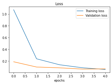
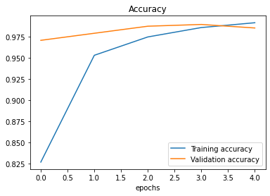
Figure 3. Accuracy and Loss of Baseline Model 1
Inspecting Trainable Layers of the EfficientNetB0 Baseline Model
We see that the efficientnetb0 layer is not tunable, while the input and output layers are adapted to our task of bird species recognition.
# Check which layers are trainable
for i, layer in enumerate(model_1.layers):
  print(i, layer.name, layer.trainable)
0 input_layer True
1 efficientnetb0 False
2 global_average_pooling True
3 output_layer True
# Summary of our baseline model 1
model_1.summary()
Model: "model"
_________________________________________________________________
 Layer (type)                Output Shape              Param #
=================================================================
 input_layer (InputLayer)    [(None, 224, 224, 3)]     0

 efficientnetb0 (Functional)  (None, None, None, 1280)  4049571

 global_average_pooling (Glo  (None, 1280)             0
 balAveragePooling2D)

 output_layer (Dense)        (None, 400)               512400

=================================================================
Total params: 4,561,971
Trainable params: 512,400
Non-trainable params: 4,049,571
_____________________________________
Evaluating the Baseline Model on the Test Dataset
Evaluating baseline model 1 on the whole test dataset gives an accuracy of 0.9845 (98.45%).
# Evaluate on the full test dataset
model_1.evaluate(test_data)
63/63 [==============================] - 5s 77ms/step - loss: 0.0611 - accuracy: 0.9845
[0.0610649473965168, 0.984499990940094]
2. EfficientNetB0 Model with Data Augmentation
We could try to further improve this result with the use of augmented data. We are not sure if data augmentation will benefit our model performance.
Creating a Keras Data Augmentation Layer (RandomFlip, RandomRotation, RandomZoom)
We can use Keras’ sequential layer for creating the data augmentation step. We performed operations such as flipping, rotating, and zooming on our birds’ images and randomly changed their width and height.
# Adding data augmentation right into the model
from tensorflow import keras
from keras import layers
from keras.layers import RandomFlip, RandomRotation, RandomZoom, RandomHeight, RandomWidth

# Create data augmentation stage with horisontal flipping, rotations, zooms, etc.
data_augmentation = keras.Sequential([
                    RandomFlip("horizontal"),
                    RandomRotation(0.2),
                    RandomZoom(0.2),
                    RandomHeight(0.2),
                    RandomWidth(0.2)
 ], name="data_augmentation")
It is always a good idea to see how the images are preprocessed.
# View a random image and compare it to its augmented version
target_class = random.choice(train_data.class_names)
target_dir = dataset_path + "/train/" + target_class
random_image = random.choice(os.listdir(target_dir))
random_image_path = target_dir + "/" + random_image
# print(random_image_path)

# Read in the random image and plot it
img = mpimg.imread(random_image_path)
plt.imshow(img)
plt.title(f"{target_class}")
plt.axis(False);

# Plotting our augmented random image
# Please note that in TF2.8 training=True is needed for the augmentation work!
augmented_img = data_augmentation(tf.squeeze(tf.expand_dims(img, axis=0)), training=True)/255.

plt.figure()
plt.imshow(augmented_img);
plt.axis(False);
plt.title(f"{target_class}");
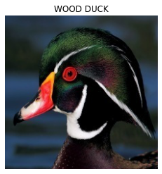
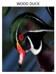
Figure 4. An Augmented Image of Wood Duck
Building Model 2 with the Augmented Data Pipeline
# Setup input shape and baseline model
# Freeze model layers
input_shape = (224, 224, 3)
baseline_model = tf.keras.applications.EfficientNetB0(include_top=False)
baseline_model.trainable = False

# Create input layer
inputs = layers.Input(shape=input_shape, name="input_layer")

# Add in data augmentation Sequential model as a layer
x = data_augmentation(inputs) # Uncomment it for data augmentation

# Give baseline_model the inputs (after augmentation) and don't train it
x = baseline_model(x, training=False)

# Pool output features of the baseline model
x = layers.GlobalAveragePooling2D(name="global_average_pooling")(x)

# Put a dense layer on as the output
outputs = layers.Dense(400, activation="softmax", name="output_layer")(x)

# Make a model using the inputs and outputs
model_2 = tf.keras.Model(inputs, outputs)

# Compile the model
model_2.compile(loss="categorical_crossentropy",
                optimizer=tf.keras.optimizers.Adam(),
                metrics=["accuracy"])

# Fit the model
history_birds_2 = model_2.fit(train_data,
                                epochs=5,
                                steps_per_epoch=len(train_data),
                                validation_data=test_data,
                                validation_steps=int(0.25*len(test_data)),
                                callbacks=[create_tensorboard_callback(dir_name="transfer_learning_birds",
                                           experiment_name="birds_baseline_data_augmentation_model_2"),
                                           create_checkpoint_callback(checkpoint_path="tmp/birds_model_2/checkpoint.ckpt")])
Saving TensorBoard log files to: transfer_learning_birds/birds_baseline_data_augmentation_model_2/20220406-13
Epoch 1/5
1825/1825 [==============================] - ETA: 0s - loss: 1.5666 - accuracy: 0.7106
1825/1825 [==============================] - 333s 179ms/step - loss: 1.5666 - accuracy: 0.7106 - val_loss: 0.3342 - val_accuracy: 0.9563
Epoch 2/5
1825/1825 [==============================] - 216s 118ms/step - loss: 0.5724 - accuracy: 0.8686 - val_loss: 0.1906 - val_accuracy: 0.9708
Epoch 3/5
1825/1825 [==============================] - 186s 102ms/step - loss: 0.4242 - accuracy: 0.8982 - val_loss: 0.1309 - val_accuracy: 0.9750
Epoch 4/5
1825/1825 [==============================] - 168s 92ms/step - loss: 0.3476 - accuracy: 0.9127 - val_loss: 0.1323 - val_accuracy: 0.9729
Epoch 5/5
1825/1825 [==============================] - 157s 86ms/step - loss: 0.2974 - accuracy: 0.9238 - val_loss: 0.1073 - val_accuracy: 0.9833
Evaluating Model 2 on the Test Dataset
Evaluating model 2 on the whole test dataset gives an accuracy of 0.9690 (96.90%).
# Evaluate on the full test dataset
model_2.evaluate(test_data)
63/63 [==============================] - 5s 70ms/step - loss: 0.1209 - accuracy: 0.9690
[0.12086006253957748, 0.968999981880188]
The model 2 performance plot shows an accuracy of 97% for the validation dataset. Interestingly, data augmentation did not help in improving model accuracy, which was lowered by 1%.
# Plot loss curves for model 2
plot_loss_curves(history_birds_2)
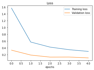
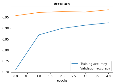
Figure 5. Accuracy and Loss of Baseline Model 2
3. Fine-Tuning Model 2 by Unfreezing the Top 10 Layers
As shown in Figure 1 above, we can do model fine-tuning after completing the feature extraction step. We build on the previous baseline model 2 with augmented data with the top layer trained on our bird species images dataset, unfreezing the top ten layers and retraining the converged model with a lower learning rate. We need to recompile the model after the model layers are unfrozen.
Feature Extraction Step Before Fine-Tuning
Firstly, we run feature extraction. This feature extraction model is identical to the previous model 2.
# Freeze model layers
baseline_model = tf.keras.applications.EfficientNetB0(include_top=False)
baseline_model.trainable = False

# Create input layer
inputs = layers.Input(shape=input_shape, name="input_layer")

# Add in data augmentation Sequential model as a layer
x = data_augmentation(inputs)

# Give baseline_model the inputs (after augmentation) and don't train it
x = baseline_model(x, training=False)

# Pool output features of the baseline model
x = layers.GlobalAveragePooling2D(name="global_average_pooling")(x)

# Put a dense layer on as the output
outputs = layers.Dense(400, activation="softmax", name="output_layer")(x)

# Make a model using the inputs and outputs
model_3 = tf.keras.Model(inputs, outputs)

# Compile the model
model_3.compile(loss="categorical_crossentropy",
                optimizer=tf.keras.optimizers.Adam(),
                metrics=["accuracy"])

# Fit the model
history_birds_3 = model_3.fit(train_data,
                                epochs=5,
                                steps_per_epoch=len(train_data),
                                validation_data=test_data,
                                validation_steps=int(0.25*len(test_data)),
                                callbacks=[create_tensorboard_callback(dir_name="transfer_learning",
                                           experiment_name="birds_baseline_data_augmentation_model_feature_extraction_3"),
                                           create_checkpoint_callback(checkpoint_path="tmp/birds_model_3/checkpoint.ckpt")])
Saving TensorBoard log files to: transfer_learning/birds_baseline_data_augmentation_model_feature_extraction_3/20220406-13
Epoch 1/5
1825/1825 [==============================] - ETA: 0s - loss: 1.5643 - accuracy: 0.7133
1825/1825 [==============================] - 161s 85ms/step - loss: 1.5643 - accuracy: 0.7133 - val_loss: 0.3349 - val_accuracy: 0.9604
Epoch 2/5
1825/1825 [==============================] - 151s 83ms/step - loss: 0.5741 - accuracy: 0.8693 - val_loss: 0.2016 - val_accuracy: 0.9667
Epoch 3/5
1825/1825 [==============================] - 148s 81ms/step - loss: 0.4275 - accuracy: 0.8964 - val_loss: 0.1257 - val_accuracy: 0.9812
Epoch 4/5
1825/1825 [==============================] - 145s 79ms/step - loss: 0.3477 - accuracy: 0.9132 - val_loss: 0.1191 - val_accuracy: 0.9708
Epoch 5/5
1825/1825 [==============================] - 144s 79ms/step - loss: 0.2985 - accuracy: 0.9232 - val_loss: 0.1122 - val_accuracy: 0.9750
As we see, the performance at this stage is identical to model 2.
# Evaluate on the full test dataset
model_3.evaluate(test_data)
63/63 [==============================] - 5s 71ms/step - loss: 0.1198 - accuracy: 0.9735
[0.11975977569818497, 0.9735000133514404]
Fine-Tuned Model 3 with a 10x Lower Learning Rate
After unfreezing the last 10 layers of the baseline model, recompile it with a lower learning rate. As suggested in the Udemy course, the learning rate could be 10 times lower then the initially defined.
# Unfreezing the last 10 layers
baseline_model.trainable = True

# Freeze all layers except for the last 10
for layer in baseline_model.layers[:-10]:
  layer.trainable = False

# Recompile our model (we have to recompile our
# model every time we make a change)
model_3.compile(loss="categorical_crossentropy",
                # When fine-tuning, we want to lower learning rate by 10x
                optimizer=keras.optimizers.Adam(learning_rate=0.0001),
                metrics=["accuracy"])
Let’s check which layers are trainable and how many trainable variables are in model 3.
# Check which layers are tunable (trainable)
for i, layer in enumerate(model_3.layers[2].layers):
  print(i, layer.name, layer.trainable)
0 input_4 False
1 rescaling_3 False
2 normalization_3 False
3 stem_conv_pad False
4 stem_conv False
5 stem_bn False
6 stem_activation False
7 block1a_dwconv False
8 block1a_bn False
9 block1a_activation False
10 block1a_se_squeeze False
11 block1a_se_reshape False
12 block1a_se_reduce False
13 block1a_se_expand False
14 block1a_se_excite False
15 block1a_project_conv False
16 block1a_project_bn False
17 block2a_expand_conv False
18 block2a_expand_bn False
19 block2a_expand_activation False
20 block2a_dwconv_pad False
21 block2a_dwconv False
22 block2a_bn False
23 block2a_activation False
24 block2a_se_squeeze False
25 block2a_se_reshape False
26 block2a_se_reduce False
27 block2a_se_expand False
28 block2a_se_excite False
29 block2a_project_conv False
30 block2a_project_bn False
31 block2b_expand_conv False
32 block2b_expand_bn False
33 block2b_expand_activation False
34 block2b_dwconv False
35 block2b_bn False
36 block2b_activation False
37 block2b_se_squeeze False
38 block2b_se_reshape False
39 block2b_se_reduce False
40 block2b_se_expand False
41 block2b_se_excite False
42 block2b_project_conv False
43 block2b_project_bn False
44 block2b_drop False
45 block2b_add False
46 block3a_expand_conv False
47 block3a_expand_bn False
48 block3a_expand_activation False
49 block3a_dwconv_pad False
50 block3a_dwconv False
51 block3a_bn False
52 block3a_activation False
53 block3a_se_squeeze False
54 block3a_se_reshape False
55 block3a_se_reduce False
56 block3a_se_expand False
57 block3a_se_excite False
58 block3a_project_conv False
59 block3a_project_bn False
60 block3b_expand_conv False
61 block3b_expand_bn False
62 block3b_expand_activation False
63 block3b_dwconv False
64 block3b_bn False
65 block3b_activation False
66 block3b_se_squeeze False
67 block3b_se_reshape False
68 block3b_se_reduce False
69 block3b_se_expand False
70 block3b_se_excite False
71 block3b_project_conv False
72 block3b_project_bn False
73 block3b_drop False
74 block3b_add False
75 block4a_expand_conv False
76 block4a_expand_bn False
77 block4a_expand_activation False
78 block4a_dwconv_pad False
79 block4a_dwconv False
80 block4a_bn False
81 block4a_activation False
82 block4a_se_squeeze False
83 block4a_se_reshape False
84 block4a_se_reduce False
85 block4a_se_expand False
86 block4a_se_excite False
87 block4a_project_conv False
88 block4a_project_bn False
89 block4b_expand_conv False
90 block4b_expand_bn False
91 block4b_expand_activation False
92 block4b_dwconv False
93 block4b_bn False
94 block4b_activation False
95 block4b_se_squeeze False
96 block4b_se_reshape False
97 block4b_se_reduce False
98 block4b_se_expand False
99 block4b_se_excite False
100 block4b_project_conv False
101 block4b_project_bn False
102 block4b_drop False
103 block4b_add False
104 block4c_expand_conv False
105 block4c_expand_bn False
106 block4c_expand_activation False
107 block4c_dwconv False
108 block4c_bn False
109 block4c_activation False
110 block4c_se_squeeze False
111 block4c_se_reshape False
112 block4c_se_reduce False
113 block4c_se_expand False
114 block4c_se_excite False
115 block4c_project_conv False
116 block4c_project_bn False
117 block4c_drop False
118 block4c_add False
119 block5a_expand_conv False
120 block5a_expand_bn False
121 block5a_expand_activation False
122 block5a_dwconv False
123 block5a_bn False
124 block5a_activation False
125 block5a_se_squeeze False
126 block5a_se_reshape False
127 block5a_se_reduce False
128 block5a_se_expand False
129 block5a_se_excite False
130 block5a_project_conv False
131 block5a_project_bn False
132 block5b_expand_conv False
133 block5b_expand_bn False
134 block5b_expand_activation False
135 block5b_dwconv False
136 block5b_bn False
137 block5b_activation False
138 block5b_se_squeeze False
139 block5b_se_reshape False
140 block5b_se_reduce False
141 block5b_se_expand False
142 block5b_se_excite False
143 block5b_project_conv False
144 block5b_project_bn False
145 block5b_drop False
146 block5b_add False
147 block5c_expand_conv False
148 block5c_expand_bn False
149 block5c_expand_activation False
150 block5c_dwconv False
151 block5c_bn False
152 block5c_activation False
153 block5c_se_squeeze False
154 block5c_se_reshape False
155 block5c_se_reduce False
156 block5c_se_expand False
157 block5c_se_excite False
158 block5c_project_conv False
159 block5c_project_bn False
160 block5c_drop False
161 block5c_add False
162 block6a_expand_conv False
163 block6a_expand_bn False
164 block6a_expand_activation False
165 block6a_dwconv_pad False
166 block6a_dwconv False
167 block6a_bn False
168 block6a_activation False
169 block6a_se_squeeze False
170 block6a_se_reshape False
171 block6a_se_reduce False
172 block6a_se_expand False
173 block6a_se_excite False
174 block6a_project_conv False
175 block6a_project_bn False
176 block6b_expand_conv False
177 block6b_expand_bn False
178 block6b_expand_activation False
179 block6b_dwconv False
180 block6b_bn False
181 block6b_activation False
182 block6b_se_squeeze False
183 block6b_se_reshape False
184 block6b_se_reduce False
185 block6b_se_expand False
186 block6b_se_excite False
187 block6b_project_conv False
188 block6b_project_bn False
189 block6b_drop False
190 block6b_add False
191 block6c_expand_conv False
192 block6c_expand_bn False
193 block6c_expand_activation False
194 block6c_dwconv False
195 block6c_bn False
196 block6c_activation False
197 block6c_se_squeeze False
198 block6c_se_reshape False
199 block6c_se_reduce False
200 block6c_se_expand False
201 block6c_se_excite False
202 block6c_project_conv False
203 block6c_project_bn False
204 block6c_drop False
205 block6c_add False
206 block6d_expand_conv False
207 block6d_expand_bn False
208 block6d_expand_activation False
209 block6d_dwconv False
210 block6d_bn False
211 block6d_activation False
212 block6d_se_squeeze False
213 block6d_se_reshape False
214 block6d_se_reduce False
215 block6d_se_expand False
216 block6d_se_excite False
217 block6d_project_conv False
218 block6d_project_bn False
219 block6d_drop False
220 block6d_add False
221 block7a_expand_conv False
222 block7a_expand_bn False
223 block7a_expand_activation False
224 block7a_dwconv False
225 block7a_bn False
226 block7a_activation False
227 block7a_se_squeeze True
228 block7a_se_reshape True
229 block7a_se_reduce True
230 block7a_se_expand True
231 block7a_se_excite True
232 block7a_project_conv True
233 block7a_project_bn True
234 top_conv True
235 top_bn True
236 top_activation True
# How many trainable variables in model_3?
len(model_3.trainable_variables)
12
Finally, we fine-tuned model 3 for another 5 epochs. We start training model at the initial epoch wherein we stopped training our feature extraction model 2.
# Fine-tune for another 5 epochs
initial_epochs = 5
fine_tune_epochs = initial_epochs +5

# Refit the model (same as model_3 except with more trainable layers)
history_model_3_fine_tuning = model_3.fit(train_data_augmented,
                                                     epochs=fine_tune_epochs,
                                                     validation_data=test_data,
                                                     validation_steps=int(0.25*len(test_data)),
                                                     # Starting from the last epoch where the model was previously left off
                                                     initial_epoch=history_birds_3.epoch[-1],
                                                     callbacks=[create_tensorboard_callback(dir_name="transfer_learning",
                                                                experiment_name="fine_tuning_birds_model_3"),
                                                                create_checkpoint_callback(checkpoint_path="tmp/birds_model_3_tuned/checkpoint.ckpt")])
Saving TensorBoard log files to: transfer_learning/fine_tuning_birds_model_3/20220406-14
Epoch 5/10
1825/1825 [==============================] - ETA: 0s - loss: 0.2071 - accuracy: 0.9443
1825/1825 [==============================] - 157s 82ms/step - loss: 0.2071 - accuracy: 0.9443 - val_loss: 0.0604 - val_accuracy: 0.9812
Epoch 6/10
1825/1825 [==============================] - 145s 79ms/step - loss: 0.1664 - accuracy: 0.9533 - val_loss: 0.0539 - val_accuracy: 0.9833
Epoch 7/10
1825/1825 [==============================] - 145s 79ms/step - loss: 0.1447 - accuracy: 0.9592 - val_loss: 0.0604 - val_accuracy: 0.9854
Epoch 8/10
1825/1825 [==============================] - 144s 79ms/step - loss: 0.1320 - accuracy: 0.9624 - val_loss: 0.0775 - val_accuracy: 0.9771
Epoch 9/10
1825/1825 [==============================] - 143s 78ms/step - loss: 0.1133 - accuracy: 0.9678 - val_loss: 0.0684 - val_accuracy: 0.9750
Epoch 10/10
1825/1825 [==============================] - 144s 79ms/step - loss: 0.1058 - accuracy: 0.9694 - val_loss: 0.0607 - val_accuracy: 0.9771
Evaluating the Fine-Tuned Model 3
Evaluating the fine-tuned model 3 on the whole test dataset gives an accuracy of 0.9740 (97.40%).
# Evaluate on the full test dataset
model_3.evaluate(test_data)
63/63 [==============================] - 5s 70ms/step - loss: 0.0750 - accuracy: 0.9740
# Plot loss curves for model 3
plot_loss_curves(history_birds_3)
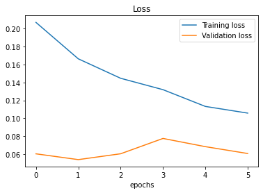
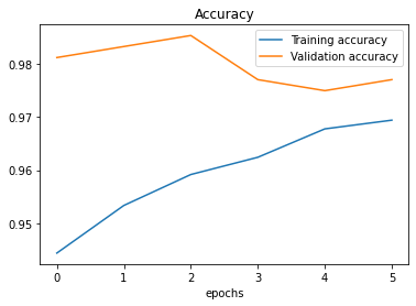
Figure 6. Accuracy and Loss of Model 3
We can compare model 2 (the feature extraction step) and model 3 (feature extraction plus fine-tuning) with the graph.
# Let's create a function to compare training histories
def compare_histories(original_history, new_history, initial_epochs=5):
  """
  Compares two TensorFlow History objects
  """

  # Get original history measurements
  accuracy = original_history.history["accuracy"]
  loss = original_history.history["loss"]

  val_accuracy = original_history.history["val_accuracy"]
  val_loss = original_history.history["val_loss"]

  # Combine original history metrics with new history metrics
  total_accuracy = accuracy + new_history.history["accuracy"]
  total_loss = loss + new_history.history["loss"]

  # Combine original history with new history metrics for validation tests
  total_val_accuracy = val_accuracy + new_history.history["val_accuracy"]
  total_val_loss = val_loss + new_history.history["val_loss"]

  # Draw plots for accuracy
  plt.figure(figsize=(8, 8))
  plt.subplot(2, 1, 1)
  plt.plot(total_accuracy, label="Training Accuracy")
  plt.plot(total_val_accuracy, label="Validation Accuracy")

  # Plot a line where the fine-tuning started
  plt.plot([initial_epochs-1, initial_epochs-1], plt.ylim(), label="Start Fine-tuning")
  plt.legend(loc="lower right")
  plt.title("Training and Validation Accuracy")


  # Draw plots for loss
  plt.figure(figsize=(8, 8))
  plt.subplot(2, 1, 2)
  plt.plot(total_loss, label="Training Loss")
  plt.plot(total_val_loss, label="Validation Loss")

  # Plot a line where the fine-tuning started
  plt.plot([initial_epochs-1, initial_epochs-1], plt.ylim(), label="Start Fine-tuning")
  plt.legend(loc="upper right")
  plt.title("Training and Validation Loss")

compare_histories(history_birds_3,
                  history_birds_3_fine_tuning,
                  initial_epochs=5)
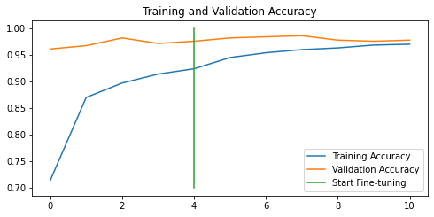
Figure 7. Performance of the Model 3: Fine-tuned
The performance of model 3, using augmented data and fine-tuned, is not much improved after further retraining with the learning rate = 0.0001.
4. Final Model 4: No Augmentation, Top 100 Layers Unfrozen
We have observed that the data augmentation step might not be helpful
with these data and models. In model 4, we build a model similar to
model 3 without a data augmentation step and unfrozen 100 top layers. The goal here is to check the
model performance and conclude on the data augmentation usefulness.
# Setup input shape and baseline model
# Freeze model layers
input_shape = (224, 224, 3)
baseline_model = tf.keras.applications.EfficientNetB0(include_top=False)
baseline_model.trainable = False

# Create input layer
inputs = layers.Input(shape=input_shape, name="input_layer")

# We remove the data augmentation step in this experiment
# x = data_augmentation(inputs)

# Give baseline_model the inputs (after augmentation) and don't train it
x = baseline_model(inputs, training=False)

# Pool output features of the baseline model
x = layers.GlobalAveragePooling2D(name="global_average_pooling")(x)

# Put a dense layer on as the output
outputs = layers.Dense(400, activation="softmax", name="output_layer")(x)

# Make a model using the inputs and outputs
model_4 = keras.Model(inputs, outputs)

# Compile the model
model_4.compile(loss="categorical_crossentropy",
                optimizer=tf.keras.optimizers.Adam(),
                metrics=["accuracy"])

# Fit the model
history_birds_4 = model_4.fit(train_data,
                                epochs=5,
                                steps_per_epoch=len(train_data),
                                validation_data=test_data,
                                validation_steps=int(0.25*len(test_data)),
                                callbacks=[create_tensorboard_callback(dir_name="transfer_learning",
                                           experiment_name="birds_baseline__feature_extraction_4"),
                                           create_checkpoint_callback(checkpoint_path="tmp/birds_model_4/checkpoint.ckpt")])
Saving TensorBoard log files to: transfer_learning/birds_baseline__feature_extraction_4/20220410-14
Epoch 1/5
1825/1825 [==============================] - 260s 138ms/step - loss: 1.0723 - accuracy: 0.8271 - val_loss: 0.1873 - val_accuracy: 0.9688
Epoch 2/5
1825/1825 [==============================] - 249s 136ms/step - loss: 0.2385 - accuracy: 0.9531 - val_loss: 0.1059 - val_accuracy: 0.9792
Epoch 3/5
1825/1825 [==============================] - 250s 137ms/step - loss: 0.1363 - accuracy: 0.9752 - val_loss: 0.0765 - val_accuracy: 0.9833
Epoch 4/5
1825/1825 [==============================] - 250s 137ms/step - loss: 0.0853 - accuracy: 0.9857 - val_loss: 0.0549 - val_accuracy: 0.9875
Epoch 5/5
1825/1825 [==============================] - 250s 137ms/step - loss: 0.0561 - accuracy: 0.9910 - val_loss: 0.0467 - val_accuracy: 0.9875
# Unfreezing the last 100 layers
baseline_model.trainable = True

# Freeze all layers except for the last 100
for layer in baseline_model.layers[:-100]:
  layer.trainable = False

# Recompile our model (we have to recompile our
# model every time we make a change)
model_4.compile(loss="categorical_crossentropy",
                # When fine-tuning, we want to lower learning rate by 10x
                optimizer=keras.optimizers.Adam(learning_rate=0.0001),
                metrics=["accuracy"])
# Fine-tune for another 5 epochs
initial_epochs = 5
fine_tune_epochs = initial_epochs +5

# Refit the model (same as model_3 except with more trainable layers)
history_model_4_fine_tuning = model_4.fit(train_data,
                                                     epochs=fine_tune_epochs,
                                                     validation_data=test_data,
                                                     validation_steps=int(0.25*len(test_data)),
                                                     # Starting from the last epoch where the model was previously left off
                                                     initial_epoch=history_birds_4.epoch[-1],
                                                     callbacks=[create_tensorboard_callback(dir_name="transfer_learning",
                                                                experiment_name="fine_tuning_birds_model_4"),
                                                                create_checkpoint_callback(checkpoint_path="tmp/birds_model_4_tuned/checkpoint.ckpt")])
Saving TensorBoard log files to: transfer_learning/fine_tuning_birds_model_4/20220413-11
Epoch 5/10
1825/1825 [==============================] - 213s 113ms/step - loss: 0.0453 - accuracy: 0.9879 - val_loss: 0.0992 - val_accuracy: 0.9750
Epoch 6/10
1825/1825 [==============================] - 204s 112ms/step - loss: 0.0238 - accuracy: 0.9934 - val_loss: 0.0773 - val_accuracy: 0.9792
Epoch 7/10
1825/1825 [==============================] - 205s 112ms/step - loss: 0.0180 - accuracy: 0.9948 - val_loss: 0.0782 - val_accuracy: 0.9812
Epoch 8/10
1825/1825 [==============================] - 204s 112ms/step - loss: 0.0152 - accuracy: 0.9956 - val_loss: 0.1045 - val_accuracy: 0.9708
Epoch 9/10
1825/1825 [==============================] - 205s 112ms/step - loss: 0.0148 - accuracy: 0.9959 - val_loss: 0.1122 - val_accuracy: 0.9708
Epoch 10/10
1825/1825 [==============================] - 205s 112ms/step - loss: 0.0119 - accuracy: 0.9965 - val_loss: 0.1034 - val_accuracy: 0.9792
# Evaluate on the full test dataset
model_4.evaluate(test_data)
63/63 [==============================] - 9s 135ms/step - loss: 0.0524 - accuracy: 0.9850
[0.05241179093718529, 0.9850000143051147]
Let’s plot accuracy and loss plots for the final model 4.
compare_histories(history_birds_4,
                  history_model_4_fine_tuning,
                  initial_epochs=5)
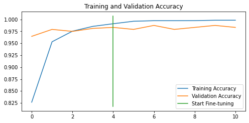
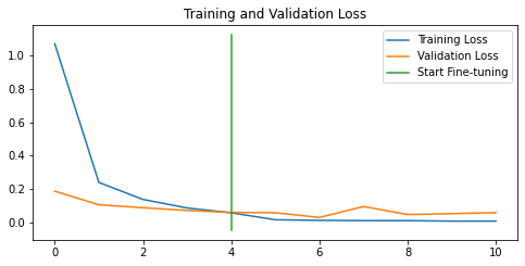
Figure 8. Performance Curves of the Model 4
To conclude, all models are well-performing, with more than 97% accuracy. We will save and zip the best-performing Model 4 for future usage in individual bird species predictions.
# Save the model 4
model_4.save("model_4")

# Zip the model 4
!zip -r model_4.zip model_4
  adding: model_4/ (stored 0%)
  adding: model_4/variables/ (stored 0%)
  adding: model_4/variables/variables.data-00000-of-00001 (deflated 8%)
  adding: model_4/variables/variables.index (deflated 74%)
  adding: model_4/assets/ (stored 0%)
  adding: model_4/keras_metadata.pb (deflated 96%)
  adding: model_4/saved_model.pb (deflated 91%)
Comparing the Four Transfer Learning Models by Accuracy
Overall, all four EfficientNetB0 transfer learning models reached more than 97% accuracy.
| Model | Configuration | Test Accuracy |
|---|---|---|
| 1. Baseline | Feature extraction, no augmentation | 0.9845 |
| 2. Baseline + Augmentation | Feature extraction with data augmentation | 0.9690 |
| 3. Fine-tuned Model 2 | Augmentation, top 10 layers unfrozen, lr=0.0001 | 0.9740 |
| 4. Final Model | No augmentation, top 100 layers unfrozen, lr=0.0001 | 0.9850 |
The final model reached slightly better accuracy, which might occur to pure chance (we did not perform statistical tests for checking if the models performance differed significantly).
# Plotting model accuracies
import pandas as pd
df = pd.DataFrame({'Model':['1. Baseline', '2. Baseline + Data Augmentation', \
                            '3. Fine-tuned Model 2', '4. Final Model'],
                   'accuracy':[0.9845, 0.9690, 0.9740, 0.9850]})
df.plot.bar(x='Model', y='accuracy', rot=45)
plt.legend(loc="lower right")
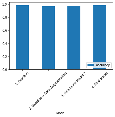
Figure 8. Four Models Compared in the Accuracy Metric
Another interesting point to consider while comparing our models is model overfitting. We can observe model overfitting when looking at the performance curves. Ideally, performance curves for training and test experiments do not have a large gap at the end of model training. For instance, Figure 3 (Model 1, the baseline) and Figure 7 (Model 3, fine-tuned) show quite a small gap between the accuracy curves. We can assume that the baseline and fine-tuned model 3 do not overfit and, therefore, might generalise very well for the unseen data. The large gap between training and test accuracy/loss curves might mean model overfitting. Figures 5 (model 2), 6 (model 3) and 8 (model 4) show that the respective models do overfit.
As you might have noticed, we used TensorBoard callbacks while training our models. This allows us to see experimental results in the TensorBoard. For this, let’s upload the results from the Colab folder into the TensorBoard. Please be aware that the results stored in the TensorBoard are all public.
!tensorboard dev upload --logdir ./transfer_learning_birds \
  --name "Transfer Learning Experiments with 400 Bird Species" \
  --description "A series of Transfer Learning Experiments with Feature Extraction and Fine-tuning." \
  --one_shot # Exits the uploader once its finished uploading
...
Done. [View your TensorBoard at https://tensorboard.dev/experiment/POgjiRKlRMO2gc2malvsjw/)
All data on TensorBoard is public, and sometimes we need to delete it knowing its ID.
# Show a list of experiments
!tensorboard dev list

# Delete an experiment
!tensorboard dev delete --experiment_id POgjiRKlRMO2gc2malvsjw
Bird Species Predictions with the Saved EfficientNetB0 Model
We observed excellent results in bird species predictions in automated tests. Let’s try to predict again with our final model that we will unzip, load from disk, evaluate with test data, and perform bird species predictions for four selected birds from our validation dataset.
# Unzipping saved model
unzip_file("/content/model_4.zip")

# Load unzipped model
loaded_model = tf.keras.models.load_model("model_4")

# Evaluate the loaded model
loaded_model.evaluate(test_data)
In the file helpers.py you can find two useful functions preprocessing and showing images in individual bird predictions. Please note that the “rescale” argument is set to False when we do not normalise bird images for further predictions. The predictive model already contains normalisation step. I have included this parameter for models which do not include a rescaling step.
# These two functions you find in the helpers.py
def load_and_prepare_image(filename, img_shape=224, rescale=True):
    """
    Preparing an image for the image prediction task.
    Reads and reshapes the tensor into the needed shape.
    Image tensor is rescaled.
    :param filename: full-path filename of the image
    :param img_shape: the required shape of the output image
    :param rescale: is True when we return normalised image tensor
    :return: image tensor
    """

    # Read the image
    img = tf.io.read_file(filename)

     # Decode the image into tensorflow
    img = tf.image.decode_image(img)

    # Resize the image
    img = tf.image.resize(img, size = [img_shape, img_shape])

    # Rescale the image
    if rescale:
        img = img/255.

    return img

def predict_and_plot(model, filename, class_names, known_label=False, rescale=True):
    """
    Loads an image stored at filename, makes the prediction,
    plots the image with the predicted class as the title.
    :param model:  Multi-class/Binary classification model.
    :param filename: filename of the image to predict.
    :param class_names: class names of the model.
    :param known_label: if we want to compare the known
    label with the predicted label.
    :param rescale: is True when we return normalised image tensor
    :return:
    """

    # import the target image and preprocess it
    img = load_and_prepare_image(filename, rescale=rescale)

    # Make a prediction
    predicted = model.predict(tf.expand_dims(img, axis=0))

    # Get the predicted class
    # Check for multi-class classification
    # print(predicted)
    if len(predicted[0])>1:
      predicted_class = class_names[tf.argmax(predicted[0])]
    else:
      # Binary classification
      predicted_class = class_names[int(tf.round(predicted[0]))]

    # Plot the image and predicted class
    plt.figure(figsize=(5,5))
    if rescale:
      plt.imshow(img);
    else:
      plt.imshow(img/255.);

    if known_label:
        if (known_label == predicted_class):
            plt.title(f"Predicted correctly: {predicted_class}")
        else:
            plt.title(f"{known_label } predicted as {predicted_class}")
    else:
        plt.title(f"Predicted: {predicted_class}")
    plt.axis(False)

filenames = ["sample_data/birds/valid/PUFFIN/2.jpg", \
             "sample_data/birds/valid/APAPANE/3.jpg", \
             "sample_data/birds/valid/AZURE JAY/2.jpg", \
             "sample_data/birds/valid/BANANAQUIT/1.jpg"]
species = ["PUFFIN", "APAPANE", "AZURE JAY", "BANANAQUIT"]

for filename, name in zip(filenames, species):
  predict_and_plot(loaded_model, filename, train_data.class_names, \
                 known_label=name, rescale=False)
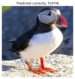
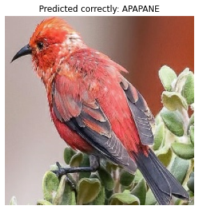
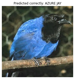
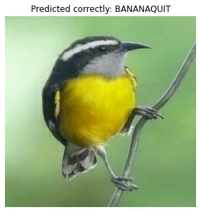
Figure 9. Four Bird Predictions
Conclusion: Fine-Tuning vs. Feature Extraction Results
Fine-tuning is a transfer learning technique that improves a converged feature extraction model by unfreezing top layers and retraining them at a 10x lower learning rate. This post built four bird species predictive models based on EfficientNetB0 from Keras using a 400-species bird dataset. The baseline feature extraction model already showed an excellent Accuracy=0.9845. Data augmentation did not improve accuracy, which slightly lowered to 0.9690. The final fine-tuned model — partially unfrozen and retrained with a lower learning rate — reached an Accuracy=0.9850. On this dataset, fine-tuning produced only a marginal gain over feature extraction, and the difference may be due to chance, since no statistical significance test was performed.
Fine-Tuning and Transfer Learning FAQ
What is fine-tuning in transfer learning?
Fine-tuning is a transfer learning method that unfreezes some layers of a pre-trained model (e.g. EfficientNetB0) and retrains them on a new dataset at a low learning rate. It adapts the learned ImageNet features to a target task such as 400-class bird species classification.
Why use a lower learning rate when fine-tuning EfficientNetB0?
Use a learning rate about 10x smaller than the feature-extraction rate (for example Adam(learning_rate=0.0001)). A small learning rate makes only minor adjustments to the pre-trained weights, preventing the model from destroying the useful ImageNet features it already learned.
How do you unfreeze layers for fine-tuning in Keras?
Set baseline_model.trainable = True, then re-freeze the lower layers in a loop: for layer in baseline_model.layers[:-10]: layer.trainable = False. You must recompile the model after changing trainable flags, then refit it from the last completed epoch.
Did data augmentation improve bird species classification accuracy?
No. On this 400 Bird Species dataset, data augmentation slightly lowered accuracy from 0.9845 (baseline) to 0.9690. The best result, 0.9850, came from the final model without augmentation and with the top 100 layers unfrozen.
References
1. TensorFlow Developer Certificate in 2022: Zero to Mastery
2. Birds 400 - Species Image Classification
5. EfficientNet: Rethinking Model Scaling for Convolutional Neural Networks
Did you like this post? Please let me know if you have any comments or suggestions.
Posts that might be interesting for youRelated Reading
Enjoyed this? Get more like it.
Weekly notes on AI tools, Python, and what I'm actually building — plus two free gifts: the 15-page Fantastic AI: The 2026 Toolkit and a Git Commands & Contribution Workflow Cheatsheet.