What Is Transfer Learning (Feature Extraction) in TensorFlow?
Previously, I have described a simple Convolutional Neural Network, which classified bird species with only 50% accuracy. The network architecture was similar to Tiny VGG and had too many parameters leading to overfitting. Image classification is a complex task. However, we can approach the problem while reusing state-of-the-art pre-trained models. Transfer learning is a machine learning technique that reuses patterns learned by a model on one dataset to improve performance on a different, related task. This way, we can efficiently apply well-tested models, potentially leading to excellent performance.
In this post, we will focus on Feature Extraction, one of the Transfer Learning techniques. I will build on the code and ideas previously shared in my previous post “Convolutional Neural Networks for Image Classification.” We will reuse previously created feature extraction models available at the TensorFlow Hub for our task of bird species recognition using image data from Kaggle. At the end of this post, we will see how this approach will improve our bird species prediction model accuracy of 50% to over 90%.
Downloading the 400 Bird Species Dataset from Kaggle
Herein, I will repeat what I have previously written how to download Kaggle datasets.
# Setup to download Kaggle datasets into a Colab instance
! pip install kaggle
! mkdir ~/.kaggle
! cp kaggle.json ~/.kaggle/
! chmod 600 ~/.kaggle/kaggle.json
! kaggle datasets download gpiosenka/100-bird-species/birds -p ./ --unzip
Let’s first import the required modules that we will use for our task.
# Importing required libraries
import tensorflow as tf
import numpy as np
import random
import matplotlib.pyplot as plt
from tensorflow.keras.optimizers import Adam
from tensorflow.keras.layers import Dense, Flatten, Conv2D, MaxPool2D, Activation
from tensorflow.keras import Sequential
from tensorflow.keras.preprocessing.image import ImageDataGenerator
import os
Visualizing the 400 Bird Species Image Data
With this code, we visualise birds from the 400 bird species dataset. The selected images have the shape of (224 pixels, 224 pixels, 3 color channels).
# Visualise our birds
import matplotlib.image as mpimg
def view_random_image(target_dir, target_class):
  # Setup the target directory
  target_folder = target_dir + target_class

  # Get a random image path
  random_image = random.sample(os.listdir(target_folder), 1)
  # print(random_image)

  # Read and plot the image
  img = mpimg.imread(target_folder + "/" + random_image[0])
  plt.imshow(img)
  plt.title(target_class)
  plt.axis("off");

  # Show the image shape
  # Uncomment this line to check image shapes
  # print(f"Image shape: {img.shape}")

  return img

dataset_path = ""

plt.figure(figsize=(20,8))
plt.subplot(2, 5, 1)
bird_img = view_random_image(dataset_path+"train/", "YELLOW CACIQUE")
plt.subplot(2, 5, 2)
bird_img = view_random_image(dataset_path+"train/", "GYRFALCON")
plt.subplot(2, 5, 3)
bird_img = view_random_image(dataset_path+"train/", "RED BEARDED BEE EATER")
plt.subplot(2, 5, 4)
bird_img = view_random_image(dataset_path+"train/", "BAIKAL TEAL")
plt.subplot(2, 5, 5)
bird_img = view_random_image(dataset_path+"train/", "DOUBLE EYED FIG PARROT")
plt.subplot(2, 5, 6)
bird_img = view_random_image(dataset_path+"train/", "STORK BILLED KINGFISHER")
plt.subplot(2, 5, 7)
bird_img = view_random_image(dataset_path+"train/", "MIKADO  PHEASANT")
plt.subplot(2, 5, 8)
bird_img = view_random_image(dataset_path+"train/", "BLUE HERON")
plt.subplot(2, 5, 9)
bird_img = view_random_image(dataset_path+"train/", "ALBATROSS")
plt.subplot(2, 5, 10)
bird_img = view_random_image(dataset_path+"train/", "RED TAILED HAWK")
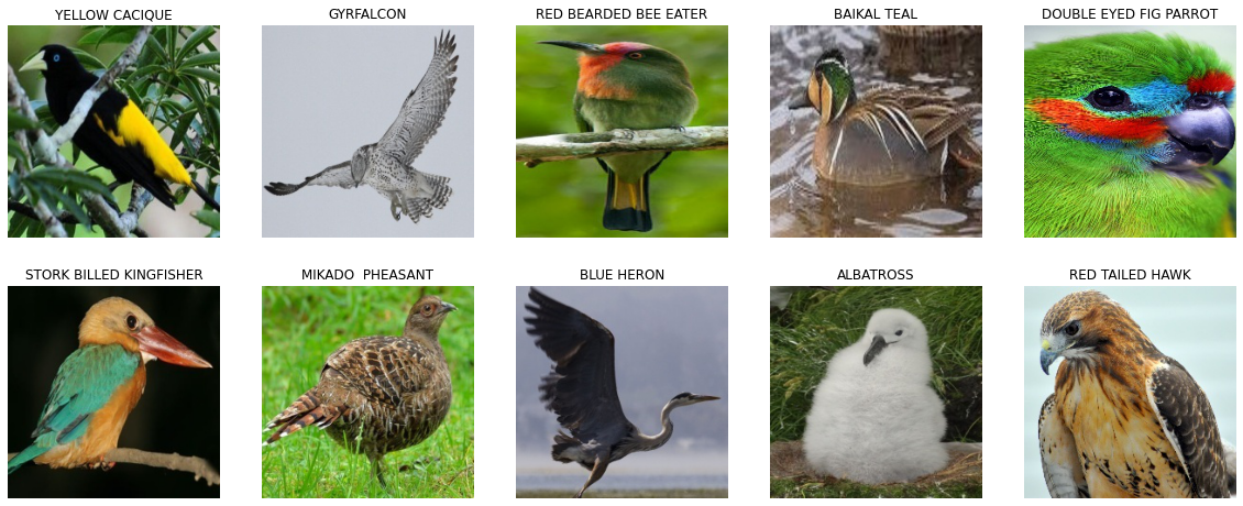
Ten birds of the Dataset
Preprocessing and Augmenting Bird Images with ImageDataGenerator
Herein we reuse the function preprocess_and_augment_data() to preprocess image data for further model training. We use image augmentation to deal with model overfitting and improve our chances of better performance on the test set. With ImageDataGenerator, bird images are rescaled, slightly rotated, zoomed, shifted, flipped, and their order is shuffled. As a result, we have our augmented training set image data stored in the variable train_data_augmented and test data (not changed) in the variable test_data. If you are interested in image data augmentation, please read the survey by Connor Shorten and Taghi M. Khoshgoftaar [6].
# Normalise training and testing data.
# Augment the training data
def preprocess_and_augment_data(train_dir, test_dir):
  # Create ImageDataGenerator training instance with data augmentation
  train_datagen_augmented = ImageDataGenerator(rescale=1/255.,
                                             rotation_range=0.2,
                                             zoom_range=0.2,
                                             width_shift_range=0.2,
                                             height_shift_range=0.2,
                                             horizontal_flip=True)

  train_data_augmented = train_datagen_augmented.flow_from_directory(dataset_path+"train/",
                                             target_size=(224, 224),
                                             batch_size=32,
                                             class_mode="categorical",
                                             shuffle=True)
  # Rescale (normalisation)
  test_datagen = ImageDataGenerator(rescale=1/255.)

  test_data = test_datagen.flow_from_directory(test_dir,
                                             target_size=(224, 224),
                                             batch_size=32,
                                             class_mode="categorical",
                                             shuffle=True)
  return train_data_augmented, test_data

train_data_augmented, test_data = preprocess_and_augment_data(train_dir=dataset_path+"train/",
                                        test_dir=dataset_path+"test/")
Found 58388 images belonging to 400 classes.
Found 2000 images belonging to 400 classes.
Feature Extraction with Pre-trained TensorFlow Hub Models
When dealing with big data, like most image datasets, we aim to reduce the data while building efficient models with less computational resources. We want not only to increase the speed of model training but also to make the model generalisable.
Since we have visual data, we employ techniques to detect shapes, lines, edges, and other image patterns. We can reuse previously trained and well-tested models for extracting image patterns with transfer learning. And the best of this approach is that we do not need to have an exact match of image categories. In feature extraction, we freeze the pre-trained base model and reuse the image features it already learned, training only a new output layer on top [7]. For our bird species recognition task, we will try to reuse image patterns extracted from the ImageNet dataset, which — per the citizen-science bird dataset paper — contains around 59 bird categories [5]. We thus extract image features using pre-trained models and further apply our own model, such as CNN in this post, for our specific image recognition task.
Where could we get already pre-trained models? Fortunately, we can get already created models from the TensorFlow Hub. I am going to follow the approach described in the Udemy course [1] while comparing transfer learning results with pre-trained ResNet and EfficientNet models.
Residual Networks (ResNet) are created for dealing with the complexity of very deep neural networks. Naturally, we expect that a deeper network leads to better model accuracy. However, He et al. observed the “degradation problem” when stacking more layers onto a very deep plain network: accuracy saturates and then degrades rapidly with depth, and this is not caused by overfitting — a deeper plain network can end up with higher training error than its shallower counterpart [9]. This is a distinct issue from the related vanishing gradient problem: the ResNet paper’s authors note that their plain deep networks, trained with batch normalisation, already showed healthy gradients, so vanishing gradients alone did not explain the degradation [9]. In ResNets [9], identity (skip) connections let a stack of layers learn a residual mapping instead of the full underlying mapping, so adding more layers never has to hurt accuracy — in the worst case, the extra layers can just learn the identity function and pass their input through unchanged [9].
# Let's compare two models
resnet_url = "https://tfhub.dev/google/imagenet/resnet_v2_50/feature_vector/5"
effecientnet_url = "https://tfhub.dev/tensorflow/efficientnet/b0/feature-vector/1"
We create and compile models using the create_model() function using these two URLs. Each model wraps a
hub.KerasLayer with trainable=False, which freezes the pre-trained weights so only our new output layer trains.
# Importing TensorFlow Hub library
import tensorflow_hub as hub

# Import layers
from tensorflow.keras import layers

# Define our image shape
IMAGE_SHAPE=(224, 224)

# Create models from a URL
def create_model(model_url, num_classes=10):
  """
  Takes a TensorFlow Hub URL and creates a Keras Sequential model with it.

  Args:
    model_url(str): A TensorFlow Hub feature extraction URL.
    num_classes(int): The number of output neurons in the output layer,
    should be equal to a number of target classes, default 10.

  Returns:
    An uncompiled Keras Sequential model with model_url as a feature extractor
    layer and Dense output layer with num_classes output neurons.
  """
  # Download the pretrained model and save it as a Keras layer
  feature_extraction_layer = hub.KerasLayer(model_url,
                                trainable=False, # Freeze the already learned patterns
                                name="feature_extraction_layer",
                                input_shape=IMAGE_SHAPE+(3, ))

  # Create our own model
  model = tf.keras.Sequential([
          feature_extraction_layer,
          layers.Dense(num_classes, activation="softmax",
                       name="output_layer")])

  # Compile  own model
  model.compile(loss="categorical_crossentropy",
                     optimizer=tf.keras.optimizers.Adam(),
                     metrics=["accuracy"])

  return model
Please note that we feed in the number of bird species classes and use “softmax” activation for the output layer.
# Create and compile Resnet Model
resnet_model = create_model(resnet_url,
                            num_classes=400)

# Create and compile EfficientNetB0 Model
effecientnet_model = create_model(effecientnet_url,
                            num_classes=400)
With plot_model(), we can draw both models. Before using plot_model, you need to have pydot and graphviz installed.
# Before using plot_model, you need to install pydot and graphviz
# I did it directly in Jupyter notebook by running the following:
# ! pip install pydot
# ! brew install graphviz
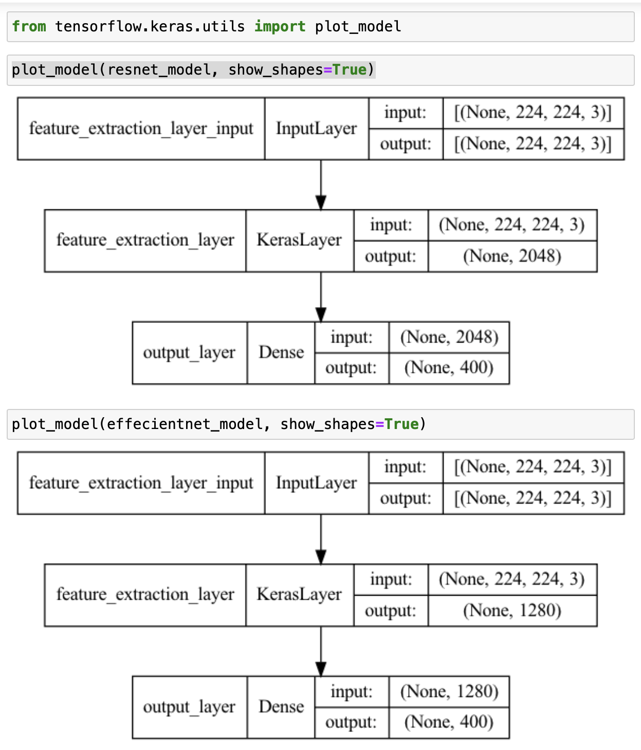
Feature Extraction Layers
Training ResNet50V2 and EfficientNetB0 Feature Extraction Models
When we build and test Machine Learning models, we are often
busy comparing different architectures and hyperparameters. We want to find
the best-performing models which generalise well. We need to keep track of the created models and
experimental results. Fortunately, we can store and monitor our performance metrics such
as accuracy and loss in TensorBoard. We will use the tf.keras.callbacks.TensorBoard callback to keep
training logs for both tested models.
# Create a function for TensorBoard callbacks
import datetime

def create_tensorboard_callback(dir_name, experiment_name):
  log_dir = dir_name + "/" + experiment_name + "/" + \
            datetime.datetime.now().strftime("%Y%m%d-%H")
  tensorboard_callback = tf.keras.callbacks.TensorBoard(log_dir=log_dir)
  print(f"Saving TensorBoard log files to: {log_dir}")
  return tensorboard_callback
Finally, we fit both models on augmented image data. Interestingly, training ResNet was about 33 minutes. EfficientNetB0 was trained in 28 minutes.
# Fit the resnet model to our data
birds_resnet_history = resnet_model.fit(train_data_augmented,
                                  epochs=5,
                                  steps_per_epoch=len(train_data_augmented),
                                  validation_data=test_data,
                                  validation_steps=len(test_data),
                                  callbacks=[create_tensorboard_callback(dir_name="tensorflow_hub",
                                                                         experiment_name="resnet50V2")])
Epoch 1/5
1825/1825 [==============================] - 349s 188ms/step - loss: 1.3401 - accuracy: 0.6940 - val_loss: 0.3167 - val_accuracy: 0.9160
Epoch 2/5
1825/1825 [==============================] - 342s 187ms/step - loss: 0.6076 - accuracy: 0.8405 - val_loss: 0.2263 - val_accuracy: 0.9355
Epoch 3/5
1825/1825 [==============================] - 342s 188ms/step - loss: 0.4973 - accuracy: 0.8648 - val_loss: 0.2173 - val_accuracy: 0.9335
Epoch 4/5
1825/1825 [==============================] - 336s 184ms/step - loss: 0.4192 - accuracy: 0.8840 - val_loss: 0.1959 - val_accuracy: 0.9445
Epoch 5/5
1825/1825 [==============================] - 333s 183ms/step - loss: 0.3731 - accuracy: 0.8957 - val_loss: 0.1744 - val_accuracy: 0.9525
# Fit the EfficientNetB0 model to our data
# It is much quicker than RestNet we trained before
birds_effecientnet_history = effecientnet_model.fit(train_data_augmented,
                                  epochs=5,
                                  steps_per_epoch=len(train_data_augmented),
                                  validation_data=test_data,
                                  validation_steps=len(test_data),
                                  callbacks=[create_tensorboard_callback(dir_name="tensorflow_hub",
                                                                         experiment_name="efficientnetB0")])
Epoch 1/5
1825/1825 [==============================] - 344s 185ms/step - loss: 1.2263 - accuracy: 0.7902 - val_loss: 0.1907 - val_accuracy: 0.9780
Epoch 2/5
1825/1825 [==============================] - 333s 182ms/step - loss: 0.3471 - accuracy: 0.9237 - val_loss: 0.1029 - val_accuracy: 0.9835
Epoch 3/5
1825/1825 [==============================] - 330s 181ms/step - loss: 0.2358 - accuracy: 0.9450 - val_loss: 0.0766 - val_accuracy: 0.9865
Epoch 4/5
1825/1825 [==============================] - 332s 182ms/step - loss: 0.1813 - accuracy: 0.9565 - val_loss: 0.0678 - val_accuracy: 0.9825
Epoch 5/5
1825/1825 [==============================] - 330s 181ms/step - loss: 0.1452 - accuracy: 0.9636 - val_loss: 0.0594 - val_accuracy: 0.9860
Comparing Loss and Accuracy Curves: ResNet vs EfficientNet
def plot_loss_curves(history):
  """
  Returns separate loss curves for training and validation matrix
  """
  loss = history.history["loss"]
  val_loss = history.history["val_loss"]

  accuracy = history.history["accuracy"]
  val_accuracy = history.history["val_accuracy"]

  epochs = range(len(history.history["loss"]))

  # Plot loss
  plt.plot(epochs, loss, label="Training loss")
  plt.plot(epochs, val_loss, label="Validation loss")
  plt.title("Loss")
  plt.xlabel("epochs")
  plt.legend()

  # Plot the accuracy
  plt.figure();
  plt.plot(epochs, accuracy, label="Training accuracy")
  plt.plot(epochs, val_accuracy, label="Validation accuracy")
  plt.title("Accuracy")
  plt.xlabel("epochs")
  plt.legend()

# Plot loss curves
plot_loss_curves(birds_resnet_history)
plot_loss_curves(birds_effecientnet_history)
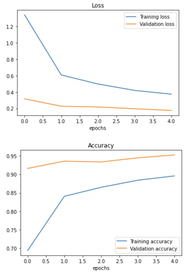
ResNet: Loss and Accuracy Plots for Bird Species Recognition
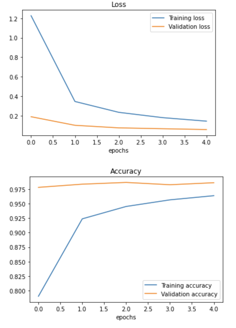
EfficientNet: Loss and Accuracy Plots for Bird Species Recognition
The EfficientNet model has higher accuracy and converges faster, it has a smaller number of total parameters.
effecientnet_model.summary()
Model: "sequential_1"
_________________________________________________________________
 Layer (type)                Output Shape              Param #
=================================================================
 feature_extraction_layer (K  (None, 1280)             4049564
 erasLayer)

 output_layer (Dense)        (None, 400)               512400

=================================================================
Total params: 4,561,964
Trainable params: 512,400
Non-trainable params: 4,049,564
_________________________________
resnet_model.summary()
Model: "sequential"
_________________________________________________________________
 Layer (type)                Output Shape              Param #
=================================================================
 feature_extraction_layer (K  (None, 2048)             23564800
 erasLayer)

 output_layer (Dense)        (None, 400)               819600

=================================================================
Total params: 24,384,400
Trainable params: 819,600
Non-trainable params: 23,564,800
Predicting Bird Species with the Trained Models
For the post completeness, I have included the code from the previous post. We use it to draw our bird species predictions using both tested models.
import pathlib
# Get the classnames programatically
def get_classnames(dataset_train_directory=dataset_path+"train/"):
  # Get the classnames programatically
  data_dir = pathlib.Path(dataset_train_directory)
  class_names = np.array(sorted([item.name for item in data_dir.glob("*")]))
  print(class_names)
  return class_names

class_names = get_classnames()

# Prepare an image for prediction
def load_and_prepare_image(filename, img_shape=224):
  """
  Preparing an image for the image prediction task.
  Reads and reshapes the tensor into the needed shape.
  """

  # Read the image
  img = tf.io.read_file(filename)

  # Decode the image into tensorflow
  img = tf.image.decode_image(img)

  # Resize the image
  img = tf.image.resize(img, size = [img_shape, img_shape])

  # Rescale the image
  img = img/255.

  return img

def predict_and_plot(model, filename, class_names, known_label=False):
    """
    Imports an image at the filename, makes the prediction,
    plots the image with the predicted class as the title.
    """

    # import the target image and preprocess it
    img = load_and_prepare_image(filename)

    # Make a prediction
    predicted = model.predict(tf.expand_dims(img, axis=0))

    # Get the predicted class
    # Check for multi-class classification
    print(predicted)
    if len(predicted[0])>1:
      predicted_class = class_names[tf.argmax(predicted[0])]
    else:
      # Binary classification
      predicted_class = class_names[int(tf.round(predicted[0]))]

    # Plot the image and predicted class
    plt.figure(figsize=(5,5))
    plt.imshow(img)
    if known_label:
        if (known_label == predicted_class):
            plt.title(f"Predicted correctly: {predicted_class}")
        else:
            plt.title(f"{known_label } predicted as {predicted_class}")
    else:
        plt.title(f"Predicted: {predicted_class}")
    plt.axis(False)
# Let's try to predict again with ResNet
predict_and_plot(resnet_model,
                 filename=dataset_path+"test/BANDED PITA/3.jpg",
                 class_names=class_names, known_label="BANDED PITA")
predict_and_plot(resnet_model,
                 filename=dataset_path+"test/BUSH TURKEY/2.jpg",
                 class_names=class_names, known_label="BUSH TURKEY")
# Let's try to predict again with EffecientNet
predict_and_plot(effecientnet_model,
                 filename=dataset_path+"test/BANDED PITA/3.jpg",
                 class_names=class_names, known_label="BANDED PITA")
predict_and_plot(effecientnet_model,
                 filename=dataset_path+"test/BUSH TURKEY/2.jpg",
                 class_names=class_names, known_label="BUSH TURKEY")
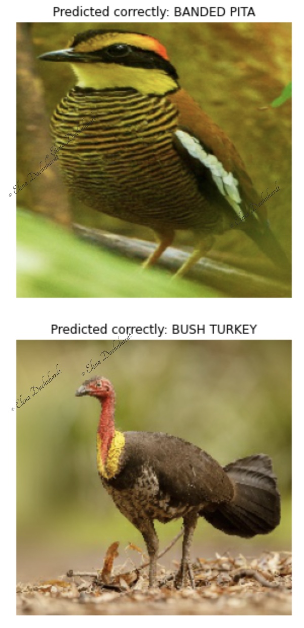
Using EfficientNet and Resnet: Bird Species Predictions with Feature Extraction
Since we had TensorBoard callback in the fit() function, we will have our training results stored in TensorBoard.
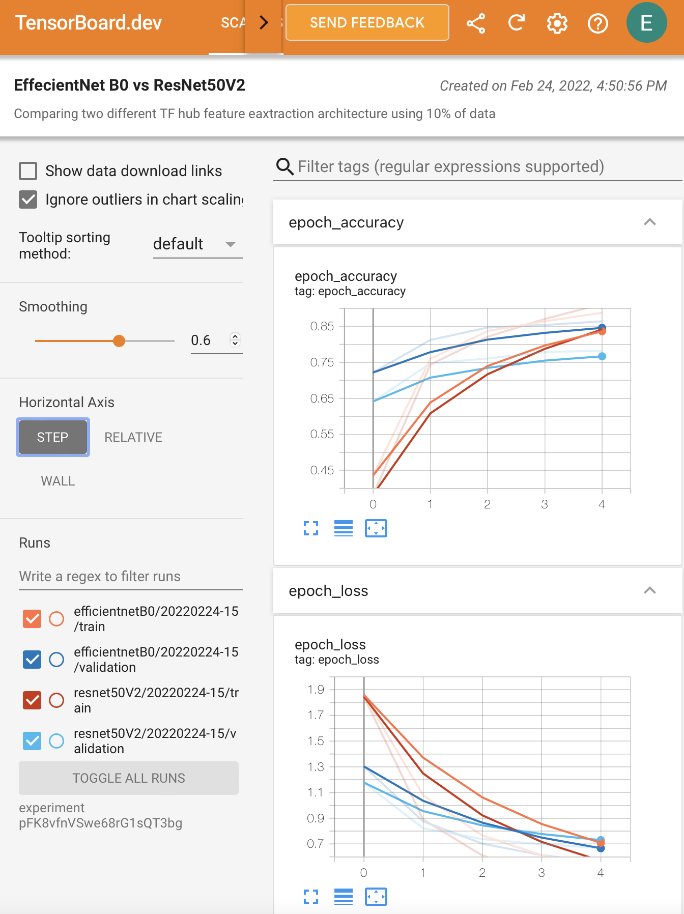
Bird Species Prediction Tests in TensorBoard
Saving and Loading a Trained Keras Model
Finally, we can reuse the improved model after saving it on disk with model.save() and reloading it with
tf.keras.models.load_model().
# Save a model
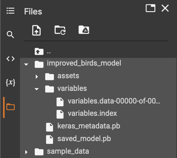
effecientnet_model.save("improved_birds_model")
# Load a model
loaded_reffecientnet_model = tf.keras.models.load_model("improved_birds_model")
# Evaluate the model on the test data
loaded_reffecientnet_model.evaluate(test_data)
We can see the improved model saved in the Colab folder.
We can zip and download the improved model to the local disk for further reuse.
# Downloading the model from Colab
!zip -r /content/improved_birds_model.zip /content/improved_birds_model

from google.colab import files
files.download('/content/improved_birds_model.zip')
   adding: content/improved_birds_model/ (stored 0%)
   adding: content/improved_birds_model/saved_model.pb (deflated 88%)
   adding: content/improved_birds_model/keras_metadata.pb (deflated 92%)
   adding: content/improved_birds_model/variables/ (stored 0%)
   adding: content/improved_birds_model/variables/variables.index (deflated 69%)
   adding: content/improved_birds_model/variables/variables.data-00000-of-00001 (deflated 13%)
   adding: content/improved_birds_model/assets/ (stored 0%)
Key Takeaways: Feature Extraction with TensorFlow Hub
Feature extraction with pre-trained TensorFlow Hub models represents a transfer learning approach that reuses frozen, pre-trained convolutional layers and trains only a new output layer, reaching high accuracy with far less data and training time than a model trained from scratch. In this post, we have built bird species recognition models using EfficientNetB0 and ResNet50V2. We achieved an accuracy of over 90% for both models exploiting pre-trained feature extraction models available at tfhub.dev. We used TensorBoard for logging our experiments and saved the improved bird species prediction model to disk.
Feature Extraction with TensorFlow Hub FAQ
What is feature extraction in transfer learning?
Feature extraction is a transfer learning technique that reuses a pre-trained model’s learned image features by freezing its layers (trainable=False) and training only a new output layer on top. It reuses patterns learned on a large dataset like ImageNet for a different classification task without retraining the whole network.
How do you freeze a pre-trained model’s layers in TensorFlow Hub?
Load the model with hub.KerasLayer(model_url, trainable=False), which prevents the pre-trained weights from updating during training. Stack a new Dense output layer with softmax activation and neurons matching your target classes, then compile and fit only that new layer.
Which performs better for feature extraction, ResNet or EfficientNet?
In this 400 bird species experiment, EfficientNetB0 reached about 98.6% validation accuracy in 28 minutes with 4.56 million total parameters, while ResNet50V2 reached about 95.25% validation accuracy in 33 minutes with 24.38 million total parameters. EfficientNet converged faster with a smaller model.
How much training data does transfer learning with feature extraction need?
Far less than training from scratch. Using ResNet50V2 and EfficientNetB0 pre-trained on ImageNet, this post reached over 90% accuracy on 400 bird species using the same 58,388-image training set that a custom CNN trained from scratch reached only about 50% accuracy on.
What is the vanishing gradient problem that ResNet was designed to solve?
The vanishing gradient problem occurs when gradients become so small during backpropagation through very deep networks that earlier layers stop learning, stalling training. ResNet addresses this with identity (skip) connections, which let gradients flow directly across layers and make it possible to train much deeper networks.
References
1. TensorFlow Developer Certificate in 2022: Zero to Mastery
2. How to Load Kaggle Datasets Directly into Google Colab?
3. Birds 400 - Species Image Classification
6. A survey on Image Data Augmentation for Deep Learning
7. Keras: Transfer learning & fine-tuning (official guide)
9. Deep Residual Learning for Image Recognition (He et al., 2015)
10. hub.KerasLayer documentation
11. tf.keras.callbacks.TensorBoard documentation
12. tf.keras.Model.save documentation
13. tf.keras.models.load_model documentation
Did you like this post? Please let me know if you have any comments or suggestions.
Posts that might be interesting for youRelated Reading
Enjoyed this? Get more like it.
Weekly notes on AI tools, Python, and what I'm actually building — plus two free gifts: the 15-page Fantastic AI: The 2026 Toolkit and a Git Commands & Contribution Workflow Cheatsheet.