
Image Classification with Convolutional Neural Networks in TensorFlow
In my previous post Multiclass Classification Model, I wrote about creating classification models using TensorFlow and Fashion MNIST dataset from Keras. We used a Sequential model with several Dense layers to build a model categorising fashion items into their respective categories, such as “T-shirt/top” or “Trouser.” The dataset was already prepared for usage, and the model created was quite simple, however, quite efficient. We could further improve our model. However, in practice, we rarely have an available dataset at hand. We can generate or collect datasets. Moreover, a simple Dense layer-based Neural Network (NN) might not work well with image data. I will focus on the more appropriate NN architecture type, which best operates when dealing with image data. We also practice working with image data presented in JPG format.
What Are Convolutional Neural Networks (CNN)?
A Convolutional Neural Network (CNN) is a deep neural network architecture that learns spatial features from grid-structured data such as images by applying trainable convolutional kernels. For Deep Learning applications on image data — visual object recognition, image segmentation, and classification — the CNN architecture requires few preprocessing steps and little human involvement, because the network learns its parameters (weights) automatically. To be used with CNN, images are presented as tensors (data structures such as matrices holding numerical data for storing image pixels and their colors). For instance, tensors can be stored in a 3-dimensional matrices with RGB-color channels (Red, Green, and Blue) defined for each pixel is what we are going to explore in this article. Generally, the CNN input is presented as a tensor with a shape: (number of inputs) x (image height) x (image width) x (number of color channels).
For instance, the CNN explainer website presents a Tiny VGG neural network trained
to classify images. Per the CNN Explainer paper, the network consists of four hidden convolutional layers (organised as two convolution-convolution-pool blocks), and the input takes
pictures with a height and width of 64 pixels and three colour channels.
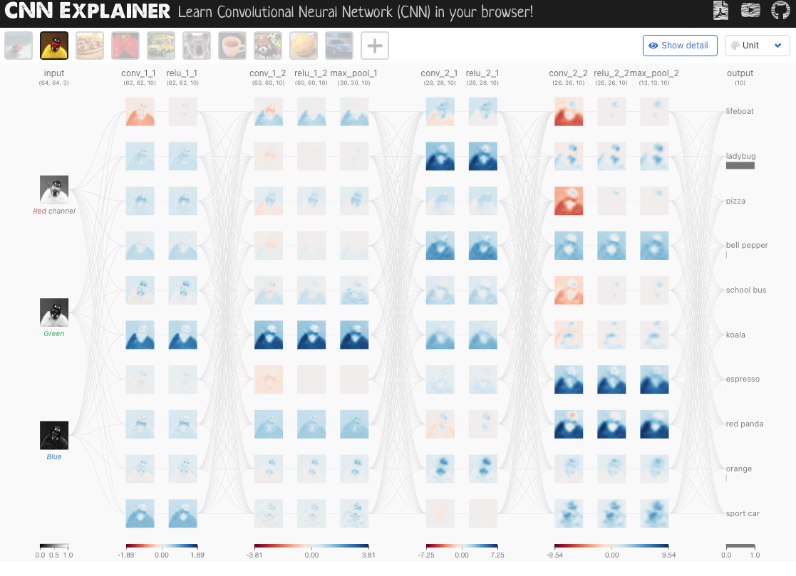
A screenshot of the CNN Explainer website at GitHub
CNN are deep networks that use hidden Convolutional layers perfectly designed for working with image data and are widely applied
in computer vision problems. Conv2D layers perform mathematical convolution operations,
which use a small matrix called “kernel” (or “filter”) applied to the input image matrix.
The smaller kernel size usually leads to better performance, while a larger kernel
learns more prominent features [1].
The CNN explainer website is interactive, and we can press on a convolution element to see how the kernel moving across its input window.
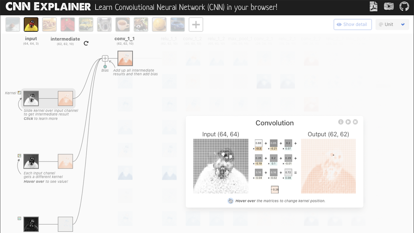
A convolution example (screenshot) at the CNN Explainer website at GitHub
The kernel moves through the image with some defined step size called “stride”; in Keras’s Conv2D the default
strides value is (1, 1), meaning “pixel by pixel”. The output of a convolutional neuron is an element-wise
dot product with the previous layer’s output and its weight, plus bias [1].
The result of such moves is an activation map. The activation map is created to extract image patterns and determine
if an image region is relevant to a specific class. The activation function is usually a “ReLU”.
ReLU fits well to non-linear data. If you are interested in activation functions, please read my post
“Artificial Neural Networks” about neural networks and some widely-used activation functions.
A CNN is a fully connected deep network. It thus operates with many parameters, which can affect negatively computational effectiveness and
even lead to overfitting (when the model “learns” training data by “heart” while failing
to work effectively with new data). This is why we can add “Pooling layers,” decreasing the spatial
extend of the network while discarding some percentage of activations. We are going to use
TensorFlow’s MaxPool2D layer, which condenses the inputs and helps find out the most essential parts of
the features found by previous convolutional layers [1].
In this post, I will reproduce an architecture similar to the Tiny VGG network. However, I will use a different Bird images dataset downloaded from Kaggle. I will also show how we can improve this model make and plot predictions. You are encouraged to further improve this model and send me your code!
Downloading the Kaggle Bird Species Dataset in Google Colab
I am using Google Colab notebooks with GPU support. You can enable the GPU with Runtime -> Change runtime type -> Hardware accelerator = GPU. For downloading Kaggle Datasets, you will need to perform a setup described by Kaustubh Gupta [2]. Herein you see the adopted code for downloading the Bird species Kaggle dataset. There are three datasets, including 58388 train, 2000 test, and 2000 validation 224x224x3 JPG images.
You can check your Nvidia information with:
!nvidia-smi
Fri Feb 18 17:16:01 2022
+-----------------------------------------------------------------------------+
| NVIDIA-SMI 460.32.03    Driver Version: 460.32.03    CUDA Version: 11.2     |
|-------------------------------+----------------------+----------------------+
| GPU  Name        Persistence-M| Bus-Id        Disp.A | Volatile Uncorr. ECC |
| Fan  Temp  Perf  Pwr:Usage/Cap|         Memory-Usage | GPU-Util  Compute M. |
|                               |                      |               MIG M. |
|===============================+======================+======================|
|   0  Tesla K80           Off  | 00000000:00:04.0 Off |                    0 |
| N/A   34C    P8    27W / 149W |      0MiB / 11441MiB |      0%      Default |
|                               |                      |                  N/A |
+-------------------------------+----------------------+----------------------+

+-----------------------------------------------------------------------------+
| Processes:                                                                  |
|  GPU   GI   CI        PID   Type   Process name                  GPU Memory |
|        ID   ID                                                   Usage      |
|=============================================================================|
|  No running processes found                                                 |
+-----------------------------------------------------------------------------+
For using Kaggle datasets, we need a Kaggle API token to be generated and downloaded in your Kaggle profile. You will need to create a Kaggle profile and go into the “Account” section. When you press the “Create New API Token,” you will get the kaggle.json file saved (it is kept in ~/Downloads for me). This JSON can be further used for all datasets. You will need to upload the kaggle.json file to the Google Colab before running the commands below.
# Setup to download Kaggle datasets into a Colab instance
! pip install kaggle
! mkdir ~/.kaggle
! cp kaggle.json ~/.kaggle/
! chmod 600 ~/.kaggle/kaggle.json
# Getting the Bird Species dataset
# Ensure that you created a folder wherein the dataset to be downloaded and unpacked
! kaggle datasets download gpiosenka/100-bird-species/birds -p /content/sample_data/birds --unzip
Downloading 100-bird-species.zip to /content/sample_data/birds
100% 1.49G/1.49G [00:16<00:00, 167MB/s]
100% 1.49G/1.49G [00:16<00:00, 95.8MB/s]
Inspecting Image Data: Counting Files and Reading Class Names
We can check how many bird images were downloaded with the code below (it shows other downloaded files). I will wrap up all further re-usable code-snips into functions.
import os

def show_file_stats(folder="sample_data/birds/"):
  # Walk thorught the directory
  for dirpath, dirnames, filenames in os.walk(folder):
    print(f"There are {len(dirnames)} directories and \
      {len(filenames)} files in '{dirpath}'.")

show_file_stats()
There are 5 directories and       5 files in 'sample_data/birds/'.
There are 400 directories and       0 files in 'sample_data/birds/valid'.
There are 0 directories and       5 files in 'sample_data/birds/valid/GROVED BILLED ANI'.
There are 0 directories and       5 files in 'sample_data/birds/valid/HOUSE SPARROW'.
There are 0 directories and       5 files in 'sample_data/birds/valid/TAILORBIRD'.
There are 0 directories and       5 files in 'sample_data/birds/valid/MALAGASY WHITE EYE'.
There are 0 directories and       5 files in 'sample_data/birds/valid/INDIAN BUSTARD'.
There are 0 directories and       5 files in 'sample_data/birds/valid/ABBOTTS BOOBY'.
There are 0 directories and       5 files in 'sample_data/birds/valid/AMERICAN PIPIT'.
....
The function get_classnames() reads a directory with train dataset to find out names of its subdirectories as classnames of bird species.
import pathlib
# Get the classnames programatically
def get_classnames(dataset_train_directory="sample_data/birds/train/"):
  # Get the classnames programatically
  data_dir = pathlib.Path(dataset_train_directory)
  class_names = np.array(sorted([item.name for item in data_dir.glob("*")]))
  print(class_names)
  return class_names

class_names = get_classnames()
['ABBOTTS BABBLER' 'ABBOTTS BOOBY' 'ABYSSINIAN GROUND HORNBILL'
 'AFRICAN CROWNED CRANE' 'AFRICAN EMERALD CUCKOO' 'AFRICAN FIREFINCH'
 'AFRICAN OYSTER CATCHER' 'ALBATROSS' 'ALBERTS TOWHEE'
 'ALEXANDRINE PARAKEET' 'ALPINE CHOUGH' 'ALTAMIRA YELLOWTHROAT'
 'AMERICAN AVOCET' 'AMERICAN BITTERN' 'AMERICAN COOT' 'AMERICAN GOLDFINCH'
 'AMERICAN KESTREL' 'AMERICAN PIPIT' 'AMERICAN REDSTART'
 'AMETHYST WOODSTAR' 'ANDEAN GOOSE' 'ANDEAN LAPWING' 'ANDEAN SISKIN'
 'ANHINGA' 'ANIANIAU' 'ANNAS HUMMINGBIRD' 'ANTBIRD' 'ANTILLEAN EUPHONIA'
 'APAPANE' 'APOSTLEBIRD' 'ARARIPE MANAKIN' 'ASHY THRUSHBIRD'
 'ASIAN CRESTED IBIS' 'AVADAVAT' 'AZURE JAY' 'AZURE TANAGER' 'AZURE TIT'
 'BAIKAL TEAL' 'BALD EAGLE' 'BALD IBIS' 'BALI STARLING' 'BALTIMORE ORIOLE'
 'BANANAQUIT' 'BAND TAILED GUAN' 'BANDED BROADBILL' 'BANDED PITA'
 'BANDED STILT' 'BAR-TAILED GODWIT' 'BARN OWL' 'BARN SWALLOW'
 'BARRED PUFFBIRD' 'BARROWS GOLDENEYE' 'BAY-BREASTED WARBLER'
 'BEARDED BARBET' 'BEARDED BELLBIRD' 'BEARDED REEDLING'
 'BELTED KINGFISHER' 'BIRD OF PARADISE' 'BLACK & YELLOW  BROADBILL'
 'BLACK BAZA' 'BLACK COCKATO' 'BLACK FRANCOLIN' 'BLACK SKIMMER'
 'BLACK SWAN' 'BLACK TAIL CRAKE' 'BLACK THROATED BUSHTIT'
 'BLACK THROATED WARBLER' 'BLACK VULTURE' 'BLACK-CAPPED CHICKADEE'
 'BLACK-NECKED GREBE' 'BLACK-THROATED SPARROW' 'BLACKBURNIAM WARBLER'
 'BLONDE CRESTED WOODPECKER' 'BLUE COAU' 'BLUE GROUSE' 'BLUE HERON'
 'BLUE THROATED TOUCANET' 'BOBOLINK' 'BORNEAN BRISTLEHEAD'
 'BORNEAN LEAFBIRD' 'BORNEAN PHEASANT' 'BRANDT CORMARANT' 'BROWN CREPPER'
 'BROWN NOODY' 'BROWN THRASHER' 'BULWERS PHEASANT' 'BUSH TURKEY'
 'CACTUS WREN' 'CALIFORNIA CONDOR' 'CALIFORNIA GULL' 'CALIFORNIA QUAIL'
 'CANARY' 'CAPE GLOSSY STARLING' 'CAPE LONGCLAW' 'CAPE MAY WARBLER'
 'CAPE ROCK THRUSH' 'CAPPED HERON' 'CAPUCHINBIRD' 'CARMINE BEE-EATER'
 'CASPIAN TERN' 'CASSOWARY' 'CEDAR WAXWING' 'CERULEAN WARBLER'
 'CHARA DE COLLAR' 'CHATTERING LORY' 'CHESTNET BELLIED EUPHONIA'
 'CHINESE BAMBOO PARTRIDGE' 'CHINESE POND HERON' 'CHIPPING SPARROW'
 'CHUCAO TAPACULO' 'CHUKAR PARTRIDGE' 'CINNAMON ATTILA'
 'CINNAMON FLYCATCHER' 'CINNAMON TEAL' 'CLARKS NUTCRACKER'
 'COCK OF THE  ROCK' 'COCKATOO' 'COLLARED ARACARI' 'COMMON FIRECREST'
 'COMMON GRACKLE' 'COMMON HOUSE MARTIN' 'COMMON IORA' 'COMMON LOON'
 'COMMON POORWILL' 'COMMON STARLING' 'COPPERY TAILED COUCAL' 'CRAB PLOVER'
 'CRANE HAWK' 'CREAM COLORED WOODPECKER' 'CRESTED AUKLET'
 'CRESTED CARACARA' 'CRESTED COUA' 'CRESTED FIREBACK' 'CRESTED KINGFISHER'
 'CRESTED NUTHATCH' 'CRESTED OROPENDOLA' 'CRESTED SHRIKETIT'
 'CRIMSON CHAT' 'CRIMSON SUNBIRD' 'CROW' 'CROWNED PIGEON' 'CUBAN TODY'
 'CUBAN TROGON' 'CURL CRESTED ARACURI' 'D-ARNAUDS BARBET'
 'DARK EYED JUNCO' 'DEMOISELLE CRANE' 'DOUBLE BARRED FINCH'
 'DOUBLE BRESTED CORMARANT' 'DOUBLE EYED FIG PARROT' 'DOWNY WOODPECKER'
 'DUSKY LORY' 'EARED PITA' 'EASTERN BLUEBIRD' 'EASTERN GOLDEN WEAVER'
 'EASTERN MEADOWLARK' 'EASTERN ROSELLA' 'EASTERN TOWEE' 'ELEGANT TROGON'
 'ELLIOTS  PHEASANT' 'EMERALD TANAGER' 'EMPEROR PENGUIN' 'EMU'
 'ENGGANO MYNA' 'EURASIAN GOLDEN ORIOLE' 'EURASIAN MAGPIE'
 'EUROPEAN GOLDFINCH' 'EUROPEAN TURTLE DOVE' 'EVENING GROSBEAK'
 'FAIRY BLUEBIRD' 'FAIRY TERN' 'FIORDLAND PENGUIN' 'FIRE TAILLED MYZORNIS'
 'FLAME BOWERBIRD' 'FLAME TANAGER' 'FLAMINGO' 'FRIGATE' 'GAMBELS QUAIL'
 'GANG GANG COCKATOO' 'GILA WOODPECKER' 'GILDED FLICKER' 'GLOSSY IBIS'
 'GO AWAY BIRD' 'GOLD WING WARBLER' 'GOLDEN CHEEKED WARBLER'
 'GOLDEN CHLOROPHONIA' 'GOLDEN EAGLE' 'GOLDEN PHEASANT' 'GOLDEN PIPIT'
 'GOULDIAN FINCH' 'GRAY CATBIRD' 'GRAY KINGBIRD' 'GRAY PARTRIDGE'
 'GREAT GRAY OWL' 'GREAT JACAMAR' 'GREAT KISKADEE' 'GREAT POTOO'
 'GREATOR SAGE GROUSE' 'GREEN BROADBILL' 'GREEN JAY' 'GREEN MAGPIE'
 'GREY PLOVER' 'GROVED BILLED ANI' 'GUINEA TURACO' 'GUINEAFOWL'
 'GURNEYS PITTA' 'GYRFALCON' 'HAMMERKOP' 'HARLEQUIN DUCK'
 'HARLEQUIN QUAIL' 'HARPY EAGLE' 'HAWAIIAN GOOSE' 'HAWFINCH'
 'HELMET VANGA' 'HEPATIC TANAGER' 'HIMALAYAN BLUETAIL' 'HIMALAYAN MONAL'
 'HOATZIN' 'HOODED MERGANSER' 'HOOPOES' 'HORNBILL' 'HORNED GUAN'
 'HORNED LARK' 'HORNED SUNGEM' 'HOUSE FINCH' 'HOUSE SPARROW'
 'HYACINTH MACAW' 'IBERIAN MAGPIE' 'IBISBILL' 'IMPERIAL SHAQ' 'INCA TERN'
 'INDIAN BUSTARD' 'INDIAN PITTA' 'INDIAN ROLLER' 'INDIGO BUNTING'
 'INLAND DOTTEREL' 'IVORY GULL' 'IWI' 'JABIRU' 'JACK SNIPE'
 'JANDAYA PARAKEET' 'JAPANESE ROBIN' 'JAVA SPARROW' 'KAGU' 'KAKAPO'
 'KILLDEAR' 'KING VULTURE' 'KIWI' 'KOOKABURRA' 'LARK BUNTING'
 'LAZULI BUNTING' 'LESSER ADJUTANT' 'LILAC ROLLER' 'LITTLE AUK'
 'LONG-EARED OWL' 'MAGPIE GOOSE' 'MALABAR HORNBILL' 'MALACHITE KINGFISHER'
 'MALAGASY WHITE EYE' 'MALEO' 'MALLARD DUCK' 'MANDRIN DUCK'
 'MANGROVE CUCKOO' 'MARABOU STORK' 'MASKED BOOBY' 'MASKED LAPWING'
 'MIKADO  PHEASANT' 'MOURNING DOVE' 'MYNA' 'NICOBAR PIGEON'
 'NOISY FRIARBIRD' 'NORTHERN CARDINAL' 'NORTHERN FLICKER'
 'NORTHERN FULMAR' 'NORTHERN GANNET' 'NORTHERN GOSHAWK' 'NORTHERN JACANA'
 'NORTHERN MOCKINGBIRD' 'NORTHERN PARULA' 'NORTHERN RED BISHOP'
 'NORTHERN SHOVELER' 'OCELLATED TURKEY' 'OKINAWA RAIL'
 'ORANGE BRESTED BUNTING' 'ORIENTAL BAY OWL' 'OSPREY' 'OSTRICH' 'OVENBIRD'
 'OYSTER CATCHER' 'PAINTED BUNTING' 'PALILA' 'PARADISE TANAGER'
 'PARAKETT  AKULET' 'PARUS MAJOR' 'PATAGONIAN SIERRA FINCH' 'PEACOCK'
 'PELICAN' 'PEREGRINE FALCON' 'PHILIPPINE EAGLE' 'PINK ROBIN'
 'POMARINE JAEGER' 'PUFFIN' 'PURPLE FINCH' 'PURPLE GALLINULE'
 'PURPLE MARTIN' 'PURPLE SWAMPHEN' 'PYGMY KINGFISHER' 'QUETZAL'
 'RAINBOW LORIKEET' 'RAZORBILL' 'RED BEARDED BEE EATER'
 'RED BELLIED PITTA' 'RED BROWED FINCH' 'RED FACED CORMORANT'
 'RED FACED WARBLER' 'RED FODY' 'RED HEADED DUCK' 'RED HEADED WOODPECKER'
 'RED HONEY CREEPER' 'RED NAPED TROGON' 'RED TAILED HAWK'
 'RED TAILED THRUSH' 'RED WINGED BLACKBIRD' 'RED WISKERED BULBUL'
 'REGENT BOWERBIRD' 'RING-NECKED PHEASANT' 'ROADRUNNER' 'ROBIN'
 'ROCK DOVE' 'ROSY FACED LOVEBIRD' 'ROUGH LEG BUZZARD' 'ROYAL FLYCATCHER'
 'RUBY THROATED HUMMINGBIRD' 'RUDY KINGFISHER' 'RUFOUS KINGFISHER'
 'RUFUOS MOTMOT' 'SAMATRAN THRUSH' 'SAND MARTIN' 'SANDHILL CRANE'
 'SATYR TRAGOPAN' 'SCARLET CROWNED FRUIT DOVE' 'SCARLET IBIS'
 'SCARLET MACAW' 'SCARLET TANAGER' 'SHOEBILL' 'SHORT BILLED DOWITCHER'
 'SMITHS LONGSPUR' 'SNOWY EGRET' 'SNOWY OWL' 'SORA' 'SPANGLED COTINGA'
 'SPLENDID WREN' 'SPOON BILED SANDPIPER' 'SPOONBILL' 'SPOTTED CATBIRD'
 'SRI LANKA BLUE MAGPIE' 'STEAMER DUCK' 'STORK BILLED KINGFISHER'
 'STRAWBERRY FINCH' 'STRIPED OWL' 'STRIPPED MANAKIN' 'STRIPPED SWALLOW'
 'SUPERB STARLING' 'SWINHOES PHEASANT' 'TAILORBIRD' 'TAIWAN MAGPIE'
 'TAKAHE' 'TASMANIAN HEN' 'TEAL DUCK' 'TIT MOUSE' 'TOUCHAN'
 'TOWNSENDS WARBLER' 'TREE SWALLOW' 'TROPICAL KINGBIRD' 'TRUMPTER SWAN'
 'TURKEY VULTURE' 'TURQUOISE MOTMOT' 'UMBRELLA BIRD' 'VARIED THRUSH'
 'VENEZUELIAN TROUPIAL' 'VERMILION FLYCATHER' 'VICTORIA CROWNED PIGEON'
 'VIOLET GREEN SWALLOW' 'VIOLET TURACO' 'VULTURINE GUINEAFOWL'
 'WALL CREAPER' 'WATTLED CURASSOW' 'WATTLED LAPWING' 'WHIMBREL'
 'WHITE BROWED CRAKE' 'WHITE CHEEKED TURACO' 'WHITE NECKED RAVEN'
 'WHITE TAILED TROPIC' 'WHITE THROATED BEE EATER' 'WILD TURKEY'
 'WILSONS BIRD OF PARADISE' 'WOOD DUCK' 'YELLOW BELLIED FLOWERPECKER'
 'YELLOW CACIQUE' 'YELLOW HEADED BLACKBIRD']
We can see random images from a specific bird species directory.
# Let's first import modules we are going to use later
import tensorflow as tf
import pandas as pd
import numpy as np
from sklearn.metrics import plot_confusion_matrix
from sklearn.metrics import confusion_matrix
import itertools
import random
import matplotlib.pyplot as plt
from tensorflow.keras.optimizers import Adam
from tensorflow.keras.layers import Dense, Flatten, Conv2D, MaxPool2D, Activation
from tensorflow.keras import Sequential
import os

# Visualise our images
import matplotlib.image as mpimg
def view_random_image(target_dir, target_class):
  # Setup the target directory
  target_folder = target_dir + target_class

  # Get a random image path
  random_image = random.sample(os.listdir(target_folder), 1)
  print(random_image)

  # Read and plot the image
  img = mpimg.imread(target_folder + "/" + random_image[0])
  plt.imshow(img)
  plt.title(target_class)
  plt.axis("off");

  # Show the image shape
  print(f"Image shape: {img.shape}")

  return img
img = view_random_image(target_dir="sample_data/birds/train/", target_class="ALPINE CHOUGH")
We can create a tensor using the “img” variable or check its shape:
tf.constant(img)

# View the image shape
img.shape # width, hight, colour channels
(224, 224, 3)
Let’s draw five random images from selected training dataset directories.
plt.figure(figsize=(20,4))
plt.subplot(1, 5, 1)
bird_img = view_random_image("sample_data/birds/train/", "SHOEBILL")
plt.subplot(1, 5, 2)
bird_img = view_random_image("sample_data/birds/train/", "RED BEARDED BEE EATER")
plt.subplot(1, 5, 3)
bird_img = view_random_image("sample_data/birds/train/", "POMARINE JAEGER")
plt.subplot(1, 5, 4)
bird_img = view_random_image("sample_data/birds/train/", "WATTLED CURASSOW")
plt.subplot(1, 5, 5)
bird_img = view_random_image("sample_data/birds/train/", "STORK BILLED KINGFISHER")
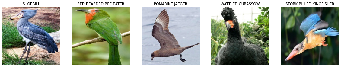
Image Preprocessing: Normalising Pixels with ImageDataGenerator
To prepare our dataset for use in CNN, we need to preprocess it. When looking into the tensor, we generated from the image provided with view_random_image() function, we can observe that our bird images consist of integer numbers from 0 to 255.
# Importing TensorFlow library
import tensorflow as tf

# Minimum and maximum value of our bird tensors
tf.constant(img).numpy().min(), tf.constant(img).numpy().max()
(0, 255)
Since neural networks work the best with scaled data, we normalise it using ImageDataGenerator taking our images directly from directories and automatically creating the training and testing datasets with categorical labels. I have wrapped the data preprocessing into the preprocess_data(rain_dir, test_dir) function.
# Import ImageDataGenerator
from tensorflow.keras.preprocessing.image import ImageDataGenerator

# Normalise training and testing data
def preprocess_data(train_dir, test_dir):
  # Rescale (normalisation)
  train_datagen = ImageDataGenerator(rescale=1/255.)
  test_datagen = ImageDataGenerator(rescale=1/255.)

  # Load data in from directories and turn it into batches
  train_data = train_datagen.flow_from_directory(train_dir,
                                               target_size=(224, 224),
                                               batch_size=32,
                                               class_mode="categorical")

  test_data = test_datagen.flow_from_directory(test_dir,
                                             target_size=(224, 224),
                                             batch_size=32,
                                             class_mode="categorical")
  return train_data, test_data

train_data, test_data = preprocess_data(train_dir="sample_data/birds/train/",
                                        test_dir="sample_data/birds/test/")
Found 58388 images belonging to 400 classes.
Found 2000 images belonging to 400 classes.
Creating and Testing CNN Models (Tiny VGG Architecture)
Above, I have referred to the Tiny VGG CNN architecture widely used as a baseline in image classification, I have replicated it with Keras NN. We use ten neurons in each Convolutional layer with the filter size of 3 and ReLU activations. Please notice that we flatten the result before feeding it into the output layer with 400 neurons and “softmax” activation since we have 400 categories or bird species.
Baseline CNN Model with Conv2D and MaxPool2D Layers
# Create our baseline model
baseline_model = Sequential([
        Conv2D(10, 3, activation="relu", input_shape=(224, 224, 3)),
        Conv2D(10, 3, activation="relu"),
        MaxPool2D(),
        Conv2D(10, 3, activation="relu"),
        Conv2D(10, 3, activation="relu"),
        MaxPool2D(),
        Flatten(),
        Dense(400, activation="softmax")
])

# Compile the model
baseline_model.compile(loss="categorical_crossentropy",
              optimizer=Adam(),
              metrics=["accuracy"])

# Fit the model
baseline_model_history = baseline_model.fit(train_data,
                            epochs=5,
                            steps_per_epoch=len(train_data),
                            validation_data=test_data,
                            validation_steps=len(test_data))
Epoch 1/5
1825/1825 [==============================] - 176s 95ms/step - loss: 4.8315 - accuracy: 0.1335 - val_loss: 3.4351 - val_accuracy: 0.3200
Epoch 2/5
1825/1825 [==============================] - 171s 94ms/step - loss: 1.5817 - accuracy: 0.6584 - val_loss: 3.6087 - val_accuracy: 0.3335
Epoch 3/5
1825/1825 [==============================] - 164s 90ms/step - loss: 0.1271 - accuracy: 0.9711 - val_loss: 6.6042 - val_accuracy: 0.2970
Epoch 4/5
1825/1825 [==============================] - 162s 89ms/step - loss: 0.0197 - accuracy: 0.9963 - val_loss: 7.7720 - val_accuracy: 0.2940
Epoch 5/5
1825/1825 [==============================] - 162s 89ms/step - loss: 0.0145 - accuracy: 0.9966 - val_loss: 8.5573 - val_accuracy: 0.2905
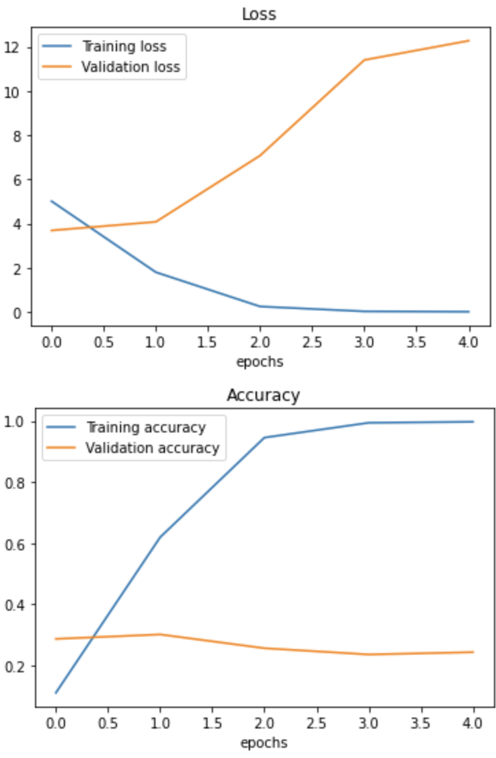
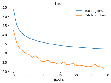
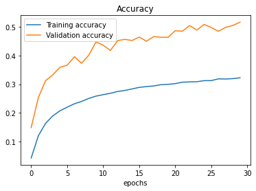
As we see from the training output, the baseline model has almost 100% accuracy on the training dataset. However, the accuracy of the test dataset is only 30%. The baseline model did not generalise well. To be sure, we can plot loss and accuracy curves. We observe significant gaps between training and test losses widening after the first training epoch. Also, the validation baseline failed to improve on the testing dataset, and the model could not generalise on unseen data.
# Plotting the loss curves using model training history data
def plot_loss_curves(history):
  """
  Returns separate loss curves for training and validation matrix
  """
  loss = history.history["loss"]
  val_loss = history.history["val_loss"]

  accuracy = history.history["accuracy"]
  val_accuracy = history.history["val_accuracy"]

  epochs = range(len(history.history["loss"]))

  # Plot loss
  plt.plot(epochs, loss, label="Training loss")
  plt.plot(epochs, val_loss, label="Validation loss")
  plt.title("Loss")
  plt.xlabel("epochs")
  plt.legend()

  # Plot the accuracy
  plt.figure();
  plt.plot(epochs, accuracy, label="Training accuracy")
  plt.plot(epochs, val_accuracy, label="Validation accuracy")
  plt.title("Accuracy")
  plt.xlabel("epochs")
  plt.legend()

plot_loss_curves(baseline_model_history)
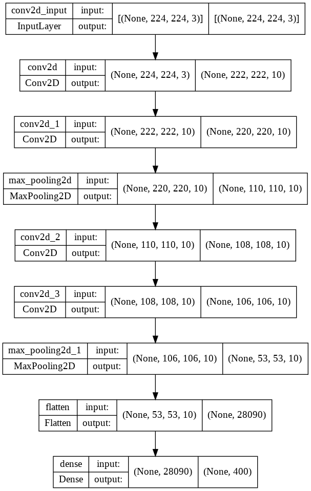
The baseline model architecture can be drawn with the plot_model function from tensorflow.keras.utils.
# Plotting deep learning models in TF
from tensorflow.keras.utils import plot_model

# See the inputs and outputs of each layer
plot_model(baseline_model, show_shapes=True)
Generating Predictions on Test Images
The accuracy and loss curves look good, but checking actual predictions matters more. The following function predict_and_plot() takes in the trained model instance and the filename of the bird image we want to predict. Please note that we need to scale and possibly, resize our input images. Therefore, we have the load_and_prepare_image() function.
# Prepare an image for prediction
def load_and_prepare_image(filename, img_shape=224):
"""
Preparing an image for image prediction task.
Reads and reshapes the tensor into needed shape.
"""
# Read the image
img = tf.io.read_file(filename)
# Decode the image into tensorflow
img = tf.image.decode_image(img)
# Resize the image
img = tf.image.resize(img, size = [img_shape, img_shape])
# Rescale the image
img = img/255.
return img
def predict_and_plot(model, filename, class_names, known_label=False):
"""
Imports an image at filename, makes the prediction,
plots the image with the predicted class as the title.
"""
# import the target image and preprocess it
img = load_and_prepare_image(filename)
# Make a prediction
predicted = model.predict(tf.expand_dims(img, axis=0))
# Get the predicted class
# Check for multi-class classification
print(predicted)
if len(predicted[0])>1:
predicted_class = class_names[tf.argmax(predicted[0])]
else:
# Binary classification
predicted_class = class_names[int(tf.round(predicted[0]))]
# Plot the image and predicted class
plt.figure(figsize=(5,5))
plt.imshow(img)
if known_label:
if (known_label == predicted_class):
plt.title(f"Predicted correctly: {predicted_class}")
else:
plt.title(f"{known_label } predicted as {predicted_class}")
else:
plt.title(f"Predicted: {predicted_class}")
plt.axis(False)
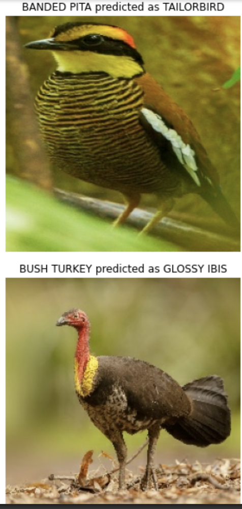
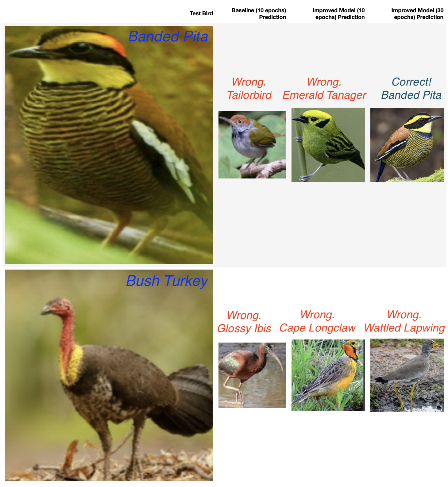
predict_and_plot(baseline_model,
filename="/content/sample_data/birds/test/ALPINE CHOUGH/2.jpg",
class_names=class_names, known_label="ALPINE CHOUGH")
predict_and_plot(baseline_model,
filename="/content/sample_data/birds/test/BANDED PITA/3.jpg",
class_names=class_names, known_label="BANDED PITA")
predict_and_plot(baseline_model,
filename="/content/sample_data/birds/test/BUSH TURKEY/2.jpg",
class_names=class_names, known_label="BUSH TURKEY")
As we see, two birds predicted wrongly; what can we do next?
Reducing CNN Overfitting with Data Augmentation
Our baseline model overfits and fails to generalise on the test data. There are many ways to improve the situation. First of all, we can collect more data, but it is not always possible. Another way is to simplify the model, for instance, by deleting neurons or hidden layers tweaking hyperparameters. Another possibility is to use transfer learning to leverage the patterns of another model learned on similar data. I will cover transfer learning in my next article. In this post, I am going to focus on data augmentation.
We process or change the data without adding more data instances when we do data augmentation. In image processing, we can flip or crop images. The data augmentation is usually performed on the trained data to bring diversity to the dataset and thus improve the generalisability of trained models.
The ImageDataGenerator class enables rescaling, image rotation, zooming, shifts, and flips, amongst other functionality.
Data augmentation happens “on the fly” and does not touch the files on disk. We do not augment the test dataset.
A note for anyone following along today: TensorFlow deprecated tf.keras.preprocessing.image.ImageDataGenerator in version 2.9, in favour of tf.keras.utils.image_dataset_from_directory combined with tf.keras.layers.RandomFlip/RandomRotation/RandomZoom preprocessing layers for augmentation. The code below still works, but if you are starting a new project, reach for the newer API.
# Improve our baseline model, which is not generalising well to
# the unseen data. The improved model should avoid the overfitting.
# We can simplify the baseline model that it does not learn
# "too much".
# Herein, we try data augmentation and fitting for longer.

# Create ImageDataGenerator training instance with data augmentation
# Normalise training and testing data.
# Augment the training data
def preprocess_and_augment_data(train_dir, test_dir):
  # Create ImageDataGenerator training instance with data augmentation
  train_datagen_augmented = ImageDataGenerator(rescale=1/255.,
                                             rotation_range=0.2,
                                             zoom_range=0.2,
                                             width_shift_range=0.2,
                                             height_shift_range=0.2,
                                             horizontal_flip=True)

  train_data_augmented = train_datagen_augmented.flow_from_directory("sample_data/birds/train/",
                                             target_size=(224, 224),
                                             batch_size=32,
                                             class_mode="categorical")
  # Rescale (normalisation)
  test_datagen = ImageDataGenerator(rescale=1/255.)

  test_data = test_datagen.flow_from_directory(test_dir,
                                             target_size=(224, 224),
                                             batch_size=32,
                                             class_mode="categorical")
  return train_data_augmented, test_data

train_data_augmented, test_data = preprocess_and_augment_data(train_dir="sample_data/birds/train/",
                                        test_dir="sample_data/birds/test/")
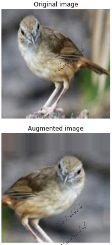
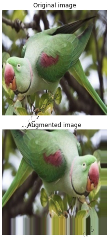
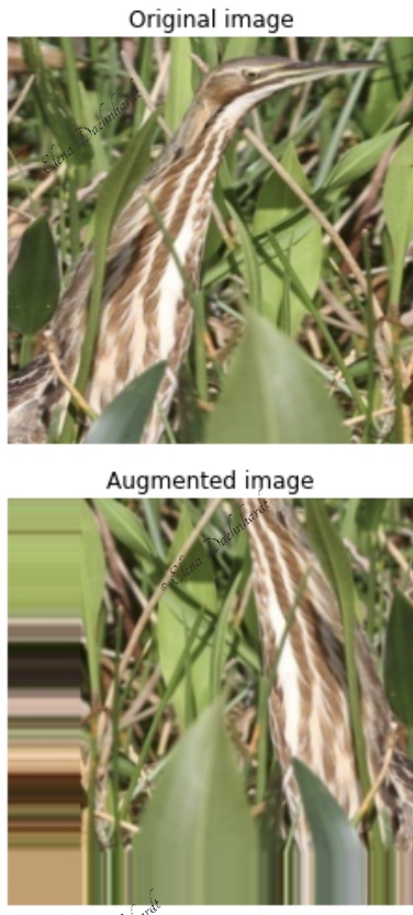
Plotting Augmented Images to Verify ImageDataGenerator
Let’s check the results of the augmentation process. Please note that this is performed on not shuffled datasets to preserve image order.
images, labels = train_data.next()
augmented_images, _ = train_data_augmented.next() # labels are not augmented

# Show the original and augmented image
# Please note that shuffle=True randomly mixxed up the images order
random_number = random.randint(0, 32)
print(f"Image number: {random_number}")
plt.imshow(images[random_number])
plt.title(f"Original image")
plt.axis(False)
plt.figure()
plt.imshow(augmented_images[random_number])
plt.title(f"Augmented image")
plt.axis(False)
Training a CNN on Augmented Data
Next, we reuse the Tiny VGG baseline model, using augmented images data and training longer.
# The model's architecture is cloned from the baseline_model, which is
# similar to the Tiny VGG model at the CNN explainer website.
# clone_model() copies the architecture with freshly initialised weights,
# it does not copy the trained weights from baseline_model [5].
improved_model = tf.keras.models.clone_model(baseline_model)

# Compile the model
improved_model.compile(loss="categorical_crossentropy",
              optimizer=Adam(),
              metrics=["accuracy"])

# Fit the model
improved_model_history = improved_model.fit(train_data_augmented,
                            epochs=30,
                            steps_per_epoch=len(train_data_augmented),
                            validation_data=test_data,
                            validation_steps=len(test_data))
# Plot loss curves
plot_loss_curves(improved_model_history)
Epoch 1/30
1825/1825 [==============================] - ETA: 0s - loss: 5.3669 - accuracy: 0.0426
1825/1825 [==============================] - 382s 209ms/step - loss: 5.3669 - accuracy: 0.0426 - val_loss: 4.2284 - val_accuracy: 0.1485
Epoch 2/30
1825/1825 [==============================] - 363s 199ms/step - loss: 4.5438 - accuracy: 0.1203 - val_loss: 3.5637 - val_accuracy: 0.2540
Epoch 3/30
1825/1825 [==============================] - 370s 203ms/step - loss: 4.2165 - accuracy: 0.1635 - val_loss: 3.2458 - val_accuracy: 0.3125
Epoch 4/30
1825/1825 [==============================] - 364s 199ms/step - loss: 4.0274 - accuracy: 0.1893 - val_loss: 3.1191 - val_accuracy: 0.3325
Epoch 5/30
1825/1825 [==============================] - 358s 196ms/step - loss: 3.9133 - accuracy: 0.2074 - val_loss: 2.9544 - val_accuracy: 0.3590
Epoch 6/30
1825/1825 [==============================] - 345s 189ms/step - loss: 3.8137 - accuracy: 0.2197 - val_loss: 2.9201 - val_accuracy: 0.3660
Epoch 7/30
1825/1825 [==============================] - 347s 190ms/step - loss: 3.7453 - accuracy: 0.2317 - val_loss: 2.7561 - val_accuracy: 0.3960
Epoch 8/30
1825/1825 [==============================] - 348s 191ms/step - loss: 3.6975 - accuracy: 0.2399 - val_loss: 2.8606 - val_accuracy: 0.3730
Epoch 9/30
1825/1825 [==============================] - 349s 191ms/step - loss: 3.6279 - accuracy: 0.2504 - val_loss: 2.7276 - val_accuracy: 0.4015
Epoch 10/30
1825/1825 [==============================] - 351s 192ms/step - loss: 3.5959 - accuracy: 0.2584 - val_loss: 2.5495 - val_accuracy: 0.4475
Epoch 11/30
1825/1825 [==============================] - 356s 195ms/step - loss: 3.5613 - accuracy: 0.2636 - val_loss: 2.5488 - val_accuracy: 0.4360
Epoch 12/30
1825/1825 [==============================] - 362s 198ms/step - loss: 3.5182 - accuracy: 0.2683 - val_loss: 2.6057 - val_accuracy: 0.4175
Epoch 13/30
1825/1825 [==============================] - 366s 200ms/step - loss: 3.4849 - accuracy: 0.2746 - val_loss: 2.4715 - val_accuracy: 0.4520
Epoch 14/30
1825/1825 [==============================] - 363s 199ms/step - loss: 3.4637 - accuracy: 0.2782 - val_loss: 2.4793 - val_accuracy: 0.4565
Epoch 15/30
1825/1825 [==============================] - 368s 202ms/step - loss: 3.4333 - accuracy: 0.2834 - val_loss: 2.4185 - val_accuracy: 0.4525
Epoch 16/30
1825/1825 [==============================] - 358s 196ms/step - loss: 3.4089 - accuracy: 0.2889 - val_loss: 2.3916 - val_accuracy: 0.4645
Epoch 17/30
1825/1825 [==============================] - 355s 194ms/step - loss: 3.3894 - accuracy: 0.2917 - val_loss: 2.5093 - val_accuracy: 0.4500
Epoch 18/30
1825/1825 [==============================] - 358s 196ms/step - loss: 3.3689 - accuracy: 0.2938 - val_loss: 2.3705 - val_accuracy: 0.4660
Epoch 19/30
1825/1825 [==============================] - 363s 199ms/step - loss: 3.3541 - accuracy: 0.2983 - val_loss: 2.3703 - val_accuracy: 0.4640
Epoch 20/30
1825/1825 [==============================] - 360s 197ms/step - loss: 3.3405 - accuracy: 0.2994 - val_loss: 2.4502 - val_accuracy: 0.4635
Epoch 21/30
1825/1825 [==============================] - 357s 196ms/step - loss: 3.3279 - accuracy: 0.3020 - val_loss: 2.3124 - val_accuracy: 0.4865
Epoch 22/30
1825/1825 [==============================] - 358s 196ms/step - loss: 3.3057 - accuracy: 0.3070 - val_loss: 2.3017 - val_accuracy: 0.4850
Epoch 23/30
1825/1825 [==============================] - 363s 199ms/step - loss: 3.2969 - accuracy: 0.3080 - val_loss: 2.3156 - val_accuracy: 0.5045
Epoch 24/30
1825/1825 [==============================] - 355s 195ms/step - loss: 3.2806 - accuracy: 0.3086 - val_loss: 2.2704 - val_accuracy: 0.4890
Epoch 25/30
1825/1825 [==============================] - 356s 195ms/step - loss: 3.2703 - accuracy: 0.3124 - val_loss: 2.2513 - val_accuracy: 0.5085
Epoch 26/30
1825/1825 [==============================] - 358s 196ms/step - loss: 3.2649 - accuracy: 0.3126 - val_loss: 2.2681 - val_accuracy: 0.4980
Epoch 27/30
1825/1825 [==============================] - 358s 196ms/step - loss: 3.2387 - accuracy: 0.3187 - val_loss: 2.3822 - val_accuracy: 0.4845
Epoch 28/30
1825/1825 [==============================] - 358s 196ms/step - loss: 3.2385 - accuracy: 0.3181 - val_loss: 2.2690 - val_accuracy: 0.4985
Epoch 29/30
1825/1825 [==============================] - 358s 196ms/step - loss: 3.2292 - accuracy: 0.3194 - val_loss: 2.2393 - val_accuracy: 0.5050
Epoch 30/30
1825/1825 [==============================] - 359s 197ms/step - loss: 3.2255 - accuracy: 0.3223 - val_loss: 2.1460 - val_accuracy: 0.5165
improved_model.summary()
Model: "sequential_1"
_________________________________________________________________
 Layer (type)                Output Shape              Param #
=================================================================
 conv2d_4 (Conv2D)           (None, 222, 222, 10)      280

 conv2d_5 (Conv2D)           (None, 220, 220, 10)      910

 max_pooling2d_2 (MaxPooling  (None, 110, 110, 10)     0
 2D)

 conv2d_6 (Conv2D)           (None, 108, 108, 10)      910

 conv2d_7 (Conv2D)           (None, 106, 106, 10)      910

 max_pooling2d_3 (MaxPooling  (None, 53, 53, 10)       0
 2D)

 flatten_1 (Flatten)         (None, 28090)             0

 dense_1 (Dense)             (None, 400)               11236400

=================================================================
Total params: 11,239,410
Trainable params: 11,239,410
Non-trainable params: 0
We observe here improved loss function and accuracy trends. However, the model is can still be further improved since the accuracy trend goes confidently up. I would try to do more training epochs.
# Let's try to predict again
predict_and_plot(improved_model,
                 filename="/content/birds/sample_data/test/BANDED PITA/3.jpg",
                 class_names=class_names, known_label="BANDED PITA")
predict_and_plot(improved_model,
                 filename="/content/birds/sample_data/test/BUSH TURKEY/2.jpg",
                 class_names=class_names, known_label="BUSH TURKEY")
One of the two images was classified wrongly. Bush Turkey was classified as Wattled Lapwing. The achieved result corresponds with our 50% accuracy, which is not suitable for practical application detection of bird species.
Conclusion: CNNs and Data Augmentation for Image Classification
In this post, I demonstrated CNN usage for bird recognition using TensorFlow (tf.keras) and the Kaggle 400 bird species dataset. We observed how the model behaves on the original and augmented images. Data augmentation is a regularisation technique that increases effective training-data diversity on the fly, reducing CNN overfitting without collecting new data. It narrowed the gap between training and test performance, though prediction accuracy after 30 epochs reached only about 50% — insufficient for practical bird-species detection. In my next post, I solve this “Turkey problem” with Transfer Learning, which classifies both birds correctly with much higher accuracy.
CNN Image Classification FAQ
Why use a CNN instead of Dense layers for image classification?
A Convolutional Neural Network (CNN) learns spatial patterns directly from pixels using shared convolutional kernels, so it needs far fewer parameters and generalises better on images than a fully-connected Dense network. Dense layers ignore spatial structure and explode in parameter count on raw images, leading to poor accuracy and overfitting.
How do you prevent overfitting in a CNN with TensorFlow?
Apply data augmentation with ImageDataGenerator (rotation, zoom, width/height shift, horizontal flip) to the training set only, add MaxPool2D layers to reduce spatial dimensions, and train for more epochs. In this post, augmentation closed the gap between ~100% training accuracy and 30% test accuracy on the baseline model, raising test accuracy to about 50%.
How do you load a Kaggle dataset into Google Colab?
Generate a Kaggle API token (kaggle.json) from your Kaggle account, upload it to Colab, then run pip install kaggle, mkdir ~/.kaggle, cp kaggle.json ~/.kaggle/, chmod 600 ~/.kaggle/kaggle.json, and kaggle datasets download <dataset> --unzip.
References
1. TensorFlow Developer Certificate in 2022: Zero to Mastery
2. How to Load Kaggle Datasets Directly into Google Colab?
3. Birds 400 - Species Image Classification
5. tf.keras.models.clone_model documentation
7. tf.keras.layers.MaxPool2D documentation
8. tf.keras.activations.relu documentation
9. tf.keras.preprocessing.image.ImageDataGenerator documentation
10. tf.keras.utils.image_dataset_from_directory documentation
11. tf.keras.utils.plot_model documentation
Did you like this post? Please let me know if you have any comments or suggestions.
Posts that might be interesting for youRelated Reading
Enjoyed this? Get more like it.
Weekly notes on AI tools, Python, and what I'm actually building — plus a free copy of Fantastic AI: The 2026 Toolkit.