What Is Multiclass Classification in TensorFlow?
Multiclass classification is a supervised learning task that assigns each input to one of three or more possible classes, in contrast to binary classification, which chooses between only two. In Machine Learning, the classification problem is categorising input data into different classes. For instance, we can categorise email messages into two groups: spam or not spam. In this case, we have two classes, we talk about binary classification. When we have more than two classes, we talk about multiclass classification. In this post, I address multiclass classification on the example of categorising clothing items into clothing types based on the Fashion MNIST dataset. The code and general concepts are adopted from TensorFlow Developer Certificate in 2022: Zero to Mastery. Below is a concise summary of the key steps: loading the data, preprocessing it, building and tuning a model, and evaluating its predictions.
Loading the Fashion MNIST Dataset in Keras
The Zalando fashion dataset is available in the tf.keras.datasets module. With the
following code, we download the dataset into training and testing datasets,
and create human-readable labels.
First of all, we need to import all required libraries.
import tensorflow as tf
import pandas as pd
import numpy as np
from sklearn.metrics import plot_confusion_matrix
from sklearn.metrics import confusion_matrix
import itertools
import random
import matplotlib.pyplot as plt
Next, we load the Fashion MNIST dataset from keras.
# Fashion dataset
fashion_mnist = tf.keras.datasets.fashion_mnist

# Get the training and testing data
(train_images, train_labels), (test_images, test_labels) = fashion_mnist.load_data()

# Create human-readable labels
class_names = ['T-shirt/top', 'Trouser', 'Pullover', 'Dress', 'Coat',
               'Sandal', 'Shirt', 'Sneaker', 'Bag', 'Ankle boot']
Downloading data from https://storage.googleapis.com/tensorflow/tf-keras-datasets/train-labels-idx1-ubyte.gz
32768/29515 [=================================] - 0s 0us/step
40960/29515 [=========================================] - 0s 0us/step
Downloading data from https://storage.googleapis.com/tensorflow/tf-keras-datasets/train-images-idx3-ubyte.gz
26427392/26421880 [==============================] - 0s 0us/step
26435584/26421880 [==============================] - 0s 0us/step
Downloading data from https://storage.googleapis.com/tensorflow/tf-keras-datasets/t10k-labels-idx1-ubyte.gz
16384/5148 [===============================================================================================] - 0s 0us/step
Downloading data from https://storage.googleapis.com/tensorflow/tf-keras-datasets/t10k-images-idx3-ubyte.gz
4423680/4422102 [==============================] - 0s 0us/step
4431872/4422102 [==============================] - 0s 0us/step
We see the shapes of downloaded training and testing datasets with their labels.
print(f"Train images shape: {train_images.shape}")
print(f"Test images shape: {test_images.shape}")
print(f"Train labels shape: {train_labels.shape}")
print(f"Test labels shape: {test_labels.shape}")
Train images shape: (60000, 28, 28)
Test images shape: (10000, 28, 28)
Train labels shape: (60000,)
Test labels shape: (10000,)
Exploring the Fashion MNIST Image Data
We observe that the dataset consists of numerical data organised into a set of 28x28 matrices with values from 0 to 255, consisting of NumPy arrays of grayscale image data. As we see from the first data row, its shape is (28, 28), the maximum value is 255.
train_images[0].shape, train_images[0].min(), train_images[0].max()
((28, 28), 0, 255)
train_images[0]
array([[  0,   0,   0,   0,   0,   0,   0,   0,   0,   0,   0,   0,   0,
          0,   0,   0,   0,   0,   0,   0,   0,   0,   0,   0,   0,   0,
          0,   0],
       [  0,   0,   0,   0,   0,   0,   0,   0,   0,   0,   0,   0,   0,
          0,   0,   0,   0,   0,   0,   0,   0,   0,   0,   0,   0,   0,
          0,   0],
       [  0,   0,   0,   0,   0,   0,   0,   0,   0,   0,   0,   0,   0,
          0,   0,   0,   0,   0,   0,   0,   0,   0,   0,   0,   0,   0,
          0,   0],
       [  0,   0,   0,   0,   0,   0,   0,   0,   0,   0,   0,   0,   1,
          0,   0,  13,  73,   0,   0,   1,   4,   0,   0,   0,   0,   1,
          1,   0],
       [  0,   0,   0,   0,   0,   0,   0,   0,   0,   0,   0,   0,   3,
          0,  36, 136, 127,  62,  54,   0,   0,   0,   1,   3,   4,   0,
          0,   3],
       [  0,   0,   0,   0,   0,   0,   0,   0,   0,   0,   0,   0,   6,
          0, 102, 204, 176, 134, 144, 123,  23,   0,   0,   0,   0,  12,
         10,   0],
       [  0,   0,   0,   0,   0,   0,   0,   0,   0,   0,   0,   0,   0,
          0, 155, 236, 207, 178, 107, 156, 161, 109,  64,  23,  77, 130,
         72,  15],
       [  0,   0,   0,   0,   0,   0,   0,   0,   0,   0,   0,   1,   0,
         69, 207, 223, 218, 216, 216, 163, 127, 121, 122, 146, 141,  88,
        172,  66],
       [  0,   0,   0,   0,   0,   0,   0,   0,   0,   1,   1,   1,   0,
        200, 232, 232, 233, 229, 223, 223, 215, 213, 164, 127, 123, 196,
        229,   0],
       [  0,   0,   0,   0,   0,   0,   0,   0,   0,   0,   0,   0,   0,
        183, 225, 216, 223, 228, 235, 227, 224, 222, 224, 221, 223, 245,
        173,   0],
       [  0,   0,   0,   0,   0,   0,   0,   0,   0,   0,   0,   0,   0,
        193, 228, 218, 213, 198, 180, 212, 210, 211, 213, 223, 220, 243,
        202,   0],
       [  0,   0,   0,   0,   0,   0,   0,   0,   0,   1,   3,   0,  12,
        219, 220, 212, 218, 192, 169, 227, 208, 218, 224, 212, 226, 197,
        209,  52],
       [  0,   0,   0,   0,   0,   0,   0,   0,   0,   0,   6,   0,  99,
        244, 222, 220, 218, 203, 198, 221, 215, 213, 222, 220, 245, 119,
        167,  56],
       [  0,   0,   0,   0,   0,   0,   0,   0,   0,   4,   0,   0,  55,
        236, 228, 230, 228, 240, 232, 213, 218, 223, 234, 217, 217, 209,
         92,   0],
       [  0,   0,   1,   4,   6,   7,   2,   0,   0,   0,   0,   0, 237,
        226, 217, 223, 222, 219, 222, 221, 216, 223, 229, 215, 218, 255,
         77,   0],
       [  0,   3,   0,   0,   0,   0,   0,   0,   0,  62, 145, 204, 228,
        207, 213, 221, 218, 208, 211, 218, 224, 223, 219, 215, 224, 244,
        159,   0],
       [  0,   0,   0,   0,  18,  44,  82, 107, 189, 228, 220, 222, 217,
        226, 200, 205, 211, 230, 224, 234, 176, 188, 250, 248, 233, 238,
        215,   0],
       [  0,  57, 187, 208, 224, 221, 224, 208, 204, 214, 208, 209, 200,
        159, 245, 193, 206, 223, 255, 255, 221, 234, 221, 211, 220, 232,
        246,   0],
       [  3, 202, 228, 224, 221, 211, 211, 214, 205, 205, 205, 220, 240,
         80, 150, 255, 229, 221, 188, 154, 191, 210, 204, 209, 222, 228,
        225,   0],
       [ 98, 233, 198, 210, 222, 229, 229, 234, 249, 220, 194, 215, 217,
        241,  65,  73, 106, 117, 168, 219, 221, 215, 217, 223, 223, 224,
        229,  29],
       [ 75, 204, 212, 204, 193, 205, 211, 225, 216, 185, 197, 206, 198,
        213, 240, 195, 227, 245, 239, 223, 218, 212, 209, 222, 220, 221,
        230,  67],
       [ 48, 203, 183, 194, 213, 197, 185, 190, 194, 192, 202, 214, 219,
        221, 220, 236, 225, 216, 199, 206, 186, 181, 177, 172, 181, 205,
        206, 115],
       [  0, 122, 219, 193, 179, 171, 183, 196, 204, 210, 213, 207, 211,
        210, 200, 196, 194, 191, 195, 191, 198, 192, 176, 156, 167, 177,
        210,  92],
       [  0,   0,  74, 189, 212, 191, 175, 172, 175, 181, 185, 188, 189,
        188, 193, 198, 204, 209, 210, 210, 211, 188, 188, 194, 192, 216,
        170,   0],
       [  2,   0,   0,   0,  66, 200, 222, 237, 239, 242, 246, 243, 244,
        221, 220, 193, 191, 179, 182, 182, 181, 176, 166, 168,  99,  58,
          0,   0],
       [  0,   0,   0,   0,   0,   0,   0,  40,  61,  44,  72,  41,  35,
          0,   0,   0,   0,   0,   0,   0,   0,   0,   0,   0,   0,   0,
          0,   0],
       [  0,   0,   0,   0,   0,   0,   0,   0,   0,   0,   0,   0,   0,
          0,   0,   0,   0,   0,   0,   0,   0,   0,   0,   0,   0,   0,
          0,   0],
       [  0,   0,   0,   0,   0,   0,   0,   0,   0,   0,   0,   0,   0,
          0,   0,   0,   0,   0,   0,   0,   0,   0,   0,   0,   0,   0,
          0,   0]], dtype=uint8)
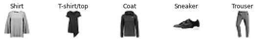
We can easily plot some of the random images in our training dataset.
# Plot an example image and its label
def plot_image(image_number=0):
  plt.imshow(train_images[image_number], cmap=plt.cm.binary)
  plt.title(class_names[train_labels[image_number]])
  plt.axis(False)

# Plot five random images
plt.figure(figsize=(10, 1))
for i in range(5):
  ax = plt.subplot(1, 5, i+1);
  rand_index = random.choice(range(len(train_images)))
  plot_image(image_number=rand_index)
Preprocessing Fashion MNIST Pixel Values for a Neural Network
As I have described in my previous post on Feature preprocessing, we need to normalise or standardise our numerical dataset. Normalising pixel values is required for training Neural Networks effectively, since they work best when input features are scaled to a small, consistent range.
# We can normalise the training and testing data
train_images_normalised = train_images / 255.0
test_images_normalised = test_images / 255.0
Building a Multiclass Classification Model in TensorFlow
When we model neural networks in TensorFlow, we generally follow the steps:
- create a model and define the input, hidden and output layers, number of neurons in each layer;
- compile the model with required loss function, optimiser, evaluation metrics;
- fit the model for finding patterns between features and labels.
Defining the Neural Network Architecture with Keras Sequential
The model architecture consists of input, hidden, and output layers. The input layer shape is defined by the number of features, while the output layer shape is defined by the number of classes. Hidden layer activation is usually ReLU, but sometimes it is good to experiment with different activations. What is an activation function? You can read my previous post Artificial Neural Networks describing some of the most useful activation functions. Our output layer activation is Softmax, good for multiclass classification problems.
# Create a model
# Use tf.one_hot(train_labels, depth=10) and tf.one_hot(test_labels, depth=10)
# with CategoricalCrossentropy()
model = tf.keras.Sequential([
        tf.keras.layers.Flatten(input_shape=(28, 28)),
        tf.keras.layers.Dense(4, activation="relu"),
        tf.keras.layers.Dense(4, activation="relu"),
        tf.keras.layers.Dense(10, activation="softmax")])
In the model compilation step, we defined the loss function. The Adam optimiser (we could also try out an SGD optimiser) works on minimising the loss function, which ideally leads to better performance. Our labels are not encoded (labels are integers). This is why we use SparseCategoricalCrossentropy. Should we try to represent our labels with a one-hot encoder, we would use CategoricalCrossentropy.
# Compile the model
model.compile(loss=tf.keras.losses.SparseCategoricalCrossentropy(),
              optimizer=tf.keras.optimizers.Adam(), metrics=["accuracy"])
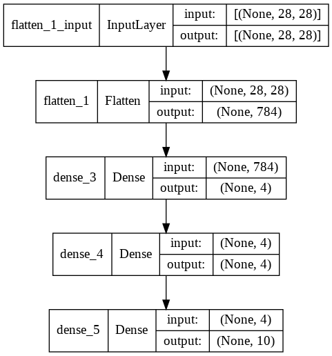
Visualizing Model Architecture with plot_model()
We can see our model architecture using the plot_model() function from tensorflow.keras.utils.
# Plotting deep learning models in TF
from tensorflow.keras.utils import plot_model

# See the inputs and outputs of each layer
plot_model(model, show_shapes=True)
Improving Model Performance: Hyperparameter Tuning Options
Even though neural networks can work out-of-the-box with default parameters pretty well, it is necessary to ensure that we have the best settings of our network hyperparameters, and also the best architecture of our network.
To improve our model, we can do the following in any combination, however, performing minor adjustments to see whether this takes any effect on the model performance 1:
- adding or removing layers;
- adding the number of hidden neurons;
- changing the activation function;
- changing the optimisation function;
- adjusting the learning rate (potentially, the most critical hyperparameter);
- adding more data;
- increasing the number of epochs;
In this post, we will focus on adjusting the learning rate with callbacks, and also define the number of epochs sufficient to get a well-performing model.
Finding the Best Learning Rate with LearningRateScheduler
During model training, we can add a callback with LearningRateScheduler to find out the best learning rate leading to the minimum loss function.
The result of the model.fit() function is find_lr_history, which keeps
the training results including loss function, accuracy for training and testing
datasets. Please note that we added validation_data for evaluating the testing dataset.
# Create the learning rate callback
lr_scheduler = tf.keras.callbacks.LearningRateScheduler(lambda epoch: 1e-3 *10**(epoch/20))

# Fit the model
find_lr_history = model.fit(train_images_normalised, train_labels,
                    epochs=40, validation_data=(test_images_normalised,
                    test_labels), callbacks=[lr_scheduler], verbose=0)
The plot below shows the loss function with respect to the learning rate. We can find out which learning rate value results in the lowest loss value.
# Plot the learning rate decay curve
lrs = 1e-3 *(10**(tf.range(40)/20))
plt.semilogx(lrs, find_lr_history.history["loss"])
plt.xlabel("Learning Rate"); plt.ylabel("Loss");
plt.title("Finding the ideal learning rate");
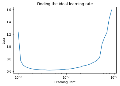
The argmin() function gives the index of the minimum loss value.
tf.argmin(find_lr_history.history["loss"])
<tf.Tensor: shape=(), dtype=int64, numpy=13>
The learning rate with the found index equals to .005, which we are going to use for building the final model.
find_lr_history.history["lr"][13]
0.004466836
# Draw the history plot with the learning rates
pd.DataFrame(find_lr_history.history).plot(figsize=(6, 4), xlabel="epochs");
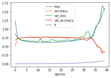
The maximum training accuracy equals about 0.8.
find_lr_history.history["accuracy"][13]
0.7751833200454712
Refitting the Model with the Best Learning Rate
In the previous step, we found out that the best learning rate for our model is .005, and the model requires 13 learning iterations.
# Create a model
# Use tf.one_hot(train_labels, depth=10) and tf.one_hot(test_labels, depth=10)
# with CategoricalCrossentropy()
model = tf.keras.Sequential([
        tf.keras.layers.Flatten(input_shape=(28, 28)),
        tf.keras.layers.Dense(4, activation="relu"),
        tf.keras.layers.Dense(4, activation="relu"),
        tf.keras.layers.Dense(10, activation="softmax")])

# Re-compile the model with the best learning rate we found
model.compile(loss=tf.keras.losses.SparseCategoricalCrossentropy(),
              optimizer=tf.keras.optimizers.Adam(lr=0.005),
              metrics=["accuracy"])

# Fit the model with the best number of epochs
history = model.fit(train_images_normalised, train_labels,
                    epochs=13, validation_data=(test_images_normalised,
                    test_labels), verbose=0)
/usr/local/lib/python3.7/dist-packages/keras/optimizer_v2/adam.py:105: UserWarning: The `lr` argument is deprecated, use `learning_rate` instead.
  super(Adam, self).__init__(name, **kwargs)
Generating Prediction Probabilities with Softmax Output
The model outputs prediction probabilities as a vector consisting of probabilities for each class label. The maximum probability corresponds to the class predicted. For instance, we predicted that the first item of our test data point corresponds to the class ‘Ankle boot.’
# Make some predictions
y_probs = model.predict(test_images_normalised)

# View the first prediction
y_probs[0], tf.argmax(y_probs[0]), class_names[tf.argmax(y_probs[0])], test_labels[0]
(array([8.8012495e-27, 7.6685532e-38, 0.0000000e+00, 1.0661165e-36,
        0.0000000e+00, 3.2718729e-02, 1.4882749e-29, 4.4392098e-02,
        4.4525089e-10, 9.2288911e-01], dtype=float32),
 <tf.Tensor: shape=(), dtype=int64, numpy=9>,
 'Ankle boot',
 9)
Using argmax(), we convert prediction probabilities into integers, which is useful since the integers are related to the class label indexes.
# Convert all of the prediction probabilities into integers
y_preds = y_probs.argmax(axis=1)

# View the first 10 prediction labels
y_preds[:10]
array([9, 4, 1, 1, 6, 1, 6, 6, 5, 7])
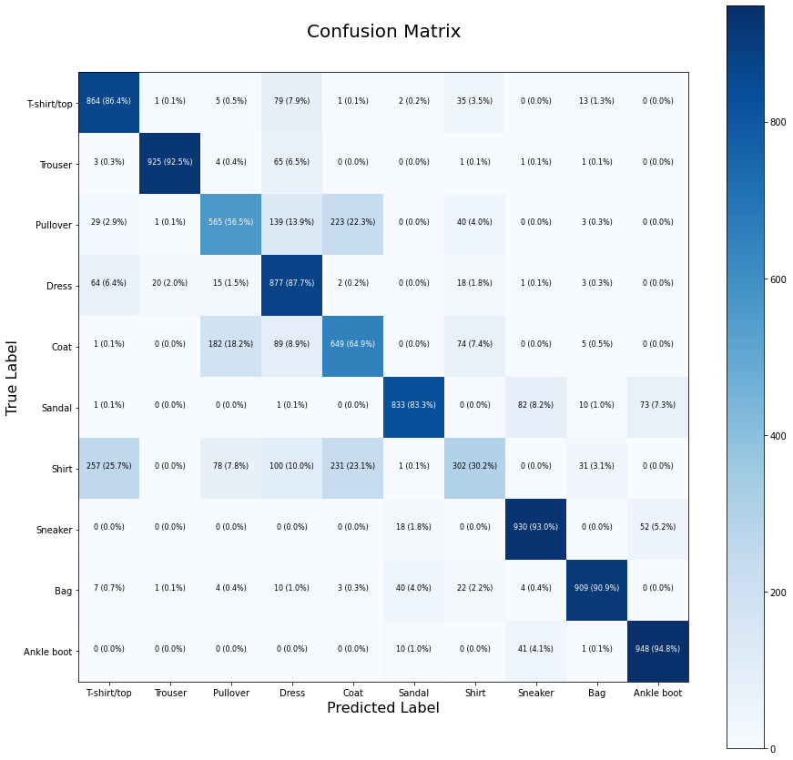
The following function provided in the Udemy course (referenced below) plots a confusion matrix using scikit-learn’s confusion_matrix function.
A confusion matrix is a table that cross-tabulates predicted labels against true labels for every class, showing the correspondence between ground truth and predictions. An ideal
confusion matrix has all values concentrated along its diagonal line.
# Plot Confusion Matrix

def plot_cm(y_test, y_preds, classes=None, figsize = (10, 10), text_size=16):
  # Create the confusion matrix
  cm = confusion_matrix(y_test, tf.round(y_preds))

  # Normalise the confusion matrix
  cm_normalised = cm.astype("float") / cm.sum(axis=1)[:, np.newaxis]

  number_of_classes = cm.shape[0]

  # Draw the plot
  fig, ax = plt.subplots(figsize=figsize)

  # Create a matrix plot
  cax = ax.matshow(cm, cmap=plt.cm.Blues)
  fig.colorbar(cax)

  # Set labels to classes
  if classes:
    labels = classes
  else:
    labels = np.arange(cm.shape[0])

  # Label the axes
  ax.set(title="Confusion Matrix",
       xlabel="Predicted Label",
       ylabel="True Label",
       xticks=np.arange(number_of_classes),
       yticks=np.arange(number_of_classes),
       xticklabels=labels,
       yticklabels=labels
       )

  # Set x-axis labels to bottom
  ax.xaxis.set_label_position("bottom")
  ax.xaxis.tick_bottom()

  # Adjust label size
  ax.yaxis.label.set_size(text_size)
  ax.xaxis.label.set_size(text_size)
  ax.title.set_size(text_size+4)

  # Set threshold for different colors
  threshold = (cm.max() + cm.min()) / 2.

  # Plot the text on each cell
  for i, j in itertools.product(range(cm.shape[0]), range(cm.shape[1])):
    plt.text(j, i, f"{cm[i, j]} ({cm_normalised[i, j]*100:.1f})",
           horizontalalignment="center",
           color="white" if cm[i, j] > threshold else "black",
           size=text_size/2)


plot_cm(test_labels, y_preds, figsize=(15, 15), classes=class_names)
Inspecting Learned Weights and Biases in Model Layers
When we train a Machine Learning model, we want it to automatically learn patterns allowing us to solve our problem, in our case, to classify fashion items. A neural network’s weights and biases are learned to get a well-performing model. Weights define the strength of the connection between neurons. Biases add constants to inputs to make the model better fit the data. We can get access to model layers as follows.
# Model layers
model.layers
[<keras.layers.core.flatten.Flatten at 0x7f3db77f3e50>,
 <keras.layers.core.dense.Dense at 0x7f3db77f32d0>,
 <keras.layers.core.dense.Dense at 0x7f3db78446d0>,
 <keras.layers.core.dense.Dense at 0x7f3db7796c50>]
# Extract a particular layer
model.layers[1]
<keras.layers.core.dense.Dense at 0x7f3db77f32d0>
Each layer has weights, and biases learned during model training.
# Get the patterns of the layer
weights, biases = model.layers[1].get_weights()

# weights and their shape
weights, weights.shape
(array([[ 0.00711583,  0.18802351, -0.92773247, -0.03165132],
        [ 1.6469412 ,  2.1759915 , -1.6559064 , -0.13926847],
        [ 1.6107311 ,  1.6976608 , -1.2488168 , -1.0657196 ],
        ...,
        [ 0.38724658,  3.3352914 ,  0.02761855, -0.6212328 ],
        [ 1.2829345 ,  1.7459874 ,  1.9171976 ,  1.2210226 ],
        [-0.04135585,  1.1622185 ,  0.5536791 ,  0.8744017 ]],
       dtype=float32), (784, 4))
# Bias and biases' shape
biases, biases.shape
(array([1.4261936, 2.5197918, 3.2453992, 4.0508494], dtype=float32), (4,))
Key Takeaways: Multiclass Classification with TensorFlow
Multiclass classification with TensorFlow’s Keras Sequential API is a repeatable workflow: load and normalise data, define a model with a Softmax output layer, use a learning-rate callback to find the optimal learning rate, then refit and evaluate with a confusion matrix. In this post, I described the multiclass classification problem using the Fashion MNIST dataset. With a training callback, I identified the best learning rate. To assess the accuracy of the classification model, I drew learning curves and a confusion matrix, and inspected the learned weights and biases of the model layers.
Multiclass Classification FAQ
What is multiclass classification in machine learning?
Multiclass classification is a supervised learning task that assigns each input to one of three or more possible classes, unlike binary classification, which chooses between only two. This post classifies Fashion MNIST images into ten clothing categories such as ‘T-shirt/top’, ‘Trouser’, and ‘Ankle boot’.
How do you find the best learning rate in TensorFlow with a callback?
Add a tf.keras.callbacks.LearningRateScheduler that increases the learning rate each epoch, e.g. lambda epoch: 1e-3 * 10**(epoch/20), fit the model, then plot loss against learning rate with plt.semilogx(). The learning rate at the lowest point of the curve — 0.005 in this experiment, found with tf.argmin(history.history['loss']) — is the best starting point for the final model.
When should I use SparseCategoricalCrossentropy instead of CategoricalCrossentropy?
Use SparseCategoricalCrossentropy when labels are plain integers, such as 3 for ‘Dress’. Use CategoricalCrossentropy when labels are one-hot encoded vectors created with tf.one_hot(labels, depth=10). Both compute the same loss; they differ only in the label format they expect.
What does the warning ‘The lr argument is deprecated, use learning_rate instead’ mean?
TensorFlow/Keras renamed the optimiser argument lr to learning_rate. Replace tf.keras.optimizers.Adam(lr=0.005) with tf.keras.optimizers.Adam(learning_rate=0.005) to silence the UserWarning and stay compatible with current Keras versions.
What does a confusion matrix show for a multiclass classification model?
A confusion matrix is a table that cross-tabulates predicted labels against true labels for every class. Each cell counts how many test examples with a given true class were predicted as each class; an ideal model has all counts concentrated on the diagonal, where predicted and true labels match.
Try the following fantastic AI-powered applications.
I am affiliated with some of them (to support my blogging at no cost to you). I have also tried these apps myself, and I liked them.
10web.io builds a website with AI. You can also host your wesbite on 10Web Hosting, and optimise it with PageSpeed Booster.
B12.io Recently, I have found an AI-powered platform that enables you to create professional websites, pages, posts, and emails with ease. I will also give it a try and soon write a new post about B12.io (I am working on my coding post at the moment :).
Mixo.io generates websites instantly using AI. Builds stunning landing pages without any code or design. Includes a built-in email waiting list and all the tools you need to launch, grow, and test your ideas.
UseBasin.com is a comprehensive backend automation platform for handling submissions, processing, filtering, and routing without coding.
Did you like this post? Please let me know if you have any comments or suggestions.
Python posts that might be interesting for youThanks
For writing this post, I have used TensorFlow documentation and tutorials at Udemy, TensorFlow Developer Certificate in 2022: Zero to Mastery.
Related Reading
Enjoyed this? Get more like it.
Weekly notes on AI tools, Python, and what I'm actually building — plus a free copy of Fantastic AI: The 2026 Toolkit.