
Feature Preprocessing for Machine Learning: One-Hot Encoding and Scaling
Feature preprocessing is the set of transformations that convert raw inputs into a form a Machine Learning algorithm can consume, applied before model training. When a dataset mixes feature types, we must prepare the data before feeding it into a Machine Learning algorithm. This happens when inputs (also called features or covariates) include categories such as gender or geographic region alongside features on different numerical scales, for instance a person’s weight or height.
A Machine Learning algorithm typically requires data in a specific type — often numerical only. ML algorithms also perform better or converge faster when data is preprocessed before training. Because the step happens before model training, we call it preprocessing. This article focuses on two main feature-preprocessing methods: feature scaling (normalisation) and feature standardisation.
Data Exploration with Pandas: info(), describe(), groupby()
To decide what we do with the data and apply Machine Learning to it, we need to analyse the dataset. We want to determine what features we have, whether they are helpful for our ML goals, how clean the dataset is, the presence of missing or noisy data. Quite often, we need also to perform data cleaning or wrangling.
Visualising features, building tables, dropping irrelevant columns, and converting data types all help here. To start playing with data, we first download our dataset — the Medical Cost Personal Datasets, originally drawn from Brett Lantz’s book Machine Learning with R and mirrored on both Kaggle and GitHub. We use the Pandas library to pull it directly from GitHub:
# Importing libraries further used in code
import pandas as pd
import matplotlib.pyplot as plt
import tensorflow as tf
insurance = pd.read_csv("https://raw.githubusercontent.com/stedy/Machine-Learning-with-R-datasets/master/insurance.csv")
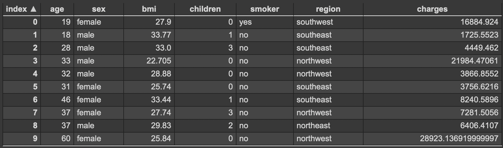
insurance.head(10)
The table shows the first ten rows of the insurance charges dataset we just downloaded. Our main goal is to predict medical insurance charges having a person’s age, sex, BMI, number of children, geographic region, and smoking status.
We can use Pandas functions such as info() and describe() to explore our features more in-depth. The info() function prints out a summary of the data with column names data types and finds any missing values.
insurance.info()
<class 'pandas.core.frame.DataFrame'>
RangeIndex: 1338 entries, 0 to 1337
Data columns (total 7 columns):
 #   Column    Non-Null Count  Dtype
---  ------    --------------  -----
 0   age       1338 non-null   int64
 1   sex       1338 non-null   object
 2   bmi       1338 non-null   float64
 3   children  1338 non-null   int64
 4   smoker    1338 non-null   object
 5   region    1338 non-null   object
 6   charges   1338 non-null   float64
dtypes: float64(2), int64(2), object(3)
memory usage: 73.3+ KB
If we need to change a data type, we use the astype() function. For instance, we want to change
the age and number of children from int64 (default type assigned when we downloaded the dataset) into int8, which
needs less memory for storage. If you are interested in playing with different data types,
read the “Overview of Pandas Data Types” by Chris Moffitt.
insurance['age']= insurance['age'].astype('int8')
insurance['children']= insurance['children'].astype('int8')
Running info() again shows we’ve already saved 18KB by switching to int8.
insurance.info()
<class 'pandas.core.frame.DataFrame'>
RangeIndex: 1338 entries, 0 to 1337
Data columns (total 7 columns):
 #   Column    Non-Null Count  Dtype
---  ------    --------------  -----
 0   age       1338 non-null   int8
 1   sex       1338 non-null   object
 2   bmi       1338 non-null   float64
 3   children  1338 non-null   int8
 4   smoker    1338 non-null   object
 5   region    1338 non-null   object
 6   charges   1338 non-null   float64
dtypes: float64(2), int8(2), object(3)
memory usage: 55.0+ KB
The describe() function is helpful for numerical features to get their statistical characteristics such as
counts, mean, standard deviation.
insurance.describe()
| index | age | bmi | children | charges |
|---|---|---|---|---|
| count | 1338.0 | 1338.0 | 1338.0 | 1338.0 |
| mean | 39.20702541106129 | 30.663396860986538 | 1.0949177877429 | 13270.422265141257 |
| std | 14.049960379216172 | 6.098186911679017 | 1.2054927397819095 | 12110.011236693994 |
| min | 18.0 | 15.96 | 0.0 | 1121.8739 |
| 25% | 27.0 | 26.29625 | 0.0 | 4740.28715 |
| 50% | 39.0 | 30.4 | 1.0 | 9382.033 |
| 75% | 51.0 | 34.69375 | 2.0 | 16639.912515 |
| max | 64.0 | 53.13 | 5.0 | 63770.42801 |
We can do further data analysis with a grouping function to observe that, on average, smokers face far larger medical insurance charges.
insurance.groupby("smoker")["charges"].mean()
smoker
no      8434.268298
yes    32050.231832
Name: charges, dtype: float64
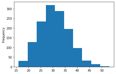
We can also draw plots with Pandas. For instance, we can plot a histogram of the “bmi” feature.
insurance["bmi"].plot(kind="hist")
Since the data exploration is not our main topic, you can read more about it at “Data Exploration 101 with Pandas” by Günter Röhrich. On possible tools to automate the data exploration, read the article by Abdishakur “4 Tools to Speed Up Exploratory Data Analysis (EDA) in Python”.
Data Preprocessing: Normalisation vs. Standardisation
To prepare our data for ML, we transform it into a more machine-readable form. For instance, we can convert string categories into numerical features and rescale numerical features with normalisation or standardisation.
Normalisation rescales data to a common range (0 to 1); scikit-learn implements it as MinMaxScaler. Standardisation removes the mean and divides each value by the standard deviation; scikit-learn implements it as StandardScaler. Both methods can improve performance or speed up convergence. The contrast between them:
| Method | scikit-learn class | Output | When to prefer |
|---|---|---|---|
| Normalisation | MinMaxScaler |
Values in [0, 1] | Neural networks; bounded inputs |
| Standardisation | StandardScaler |
Zero mean, unit variance | Linear/logistic regression, nearest neighbours, features with outliers |
Linear and logistic regression, nearest neighbours, and neural networks all benefit from feature scaling. Neural networks often do better with normalisation — but test both on your own data and see which one trains faster or scores better.
Transforming Features with MinMaxScaler and OneHotEncoder
Let’s transform features with MinMaxScaler and OneHotEncoder (scikit-learn) for our insurance charges dataset. Both methods are combined in a single preprocessing step with make_column_transformer(). We fit the column transformer on the training data only, then apply it to the testing data — this ordering prevents data leakage, where test-set statistics contaminate training. Read more in “How to Avoid Data Leakage When Performing Data Preparation” by Jason Brownlee.
from sklearn.compose import make_column_transformer
from sklearn.preprocessing import MinMaxScaler, OneHotEncoder
from sklearn.model_selection import train_test_split

# Create column transformer for feature preprocessing
column_transformer = make_column_transformer(
    (MinMaxScaler(), ["age", "bmi", "children"]),
    (OneHotEncoder(handle_unknown="ignore"), ["sex", "smoker", "region"])
)

# Create X and y
X = insurance.drop("charges", axis=1)
y = insurance["charges"]

# Build our train and test sets
X_train, X_test, y_train, y_test = train_test_split(X, y, test_size = 0.2,
                                                    random_state=57)

# Fit the column transformer to our training data
column_transformer.fit(X_train)

# Transform training and test data with normalisation (MinMaxScaler)
# and OneHotEncoder
X_train_normalised = column_transformer.transform(X_train)
X_test_normalised = column_transformer.transform(X_test)

# Normalised features example
X_train_normalised[0]
array([0.02173913, 0.34217191, 0.        , 1.        , 0.        ,
       0.        , 1.        , 0.        , 0.        , 0.        ,
       1.        ])
Creating and Evaluating a Keras Neural Network on Preprocessed Data
We build a neural network to fit the normalised, preprocessed data. We use a Keras Sequential model with two hidden ReLU layers and a single linear output neuron for regression. Evaluating the model on the test set yields MAE=1697.4192.
# Build a neural network to fit the normalised data
model = tf.keras.models.Sequential([
        tf.keras.layers.Dense(100, activation="relu"),
        tf.keras.layers.Dense(10, activation="relu"),
        tf.keras.layers.Dense(1)
])

model.compile(loss=tf.keras.losses.mae,
                 optimizer=tf.keras.optimizers.Adam(lr=0.1),
                 metrics=["mae"])

history = model.fit(X_train_normalised, y_train, epochs=100, verbose=0)

model.evaluate(X_test_normalised, y_test)
/usr/local/lib/python3.7/dist-packages/keras/optimizer_v2/adam.py:105: UserWarning: The `lr` argument is deprecated, use `learning_rate` instead.
  super(Adam, self).__init__(name, **kwargs)
9/9 [==============================] - 0s 2ms/step - loss: 1697.4192 - mae: 1697.4192
[1697.419189453125, 1697.419189453125]
Fixing “UserWarning: The lr argument is deprecated, use learning_rate instead”
This warning appears when compiling a Keras optimiser with the old lr= keyword. Cause: Keras 2.3.0 renamed the optimiser argument from lr to learning_rate for every optimiser, and later TensorFlow releases added a runtime UserWarning if you still pass the old keyword. Fix it by renaming the keyword — and do it now rather than later: I tested this on a current Keras 3 install, and lr= is no longer just deprecated, it is rejected outright with ValueError: Argument(s) not recognized: {'lr': 0.1}, since Keras 3’s optimizer base class only special-cases the decay argument for a soft warning and raises on everything else it does not recognise.
# Deprecated:
optimizer=tf.keras.optimizers.Adam(lr=0.1)

# Current:
optimizer=tf.keras.optimizers.Adam(learning_rate=0.1)
Conclusion: A One-Step Column Transformer Before Model Training
In this post, we downloaded the insurance charges dataset from GitHub and preprocessed it with the Pandas and scikit-learn libraries. scikit-learn let us combine one-hot encoding and feature scaling in a single column-transforming step performed before building the ML model. We then trained and evaluated a Keras neural network on the prepared data. A make_column_transformer pipeline fitted on training data only is the standard scikit-learn pattern for preprocessing mixed numerical and categorical features without data leakage.
Feature Preprocessing FAQ
What is the difference between normalisation and standardisation?
Normalisation rescales features to a fixed range (typically 0 to 1) using scikit-learn’s MinMaxScaler. Standardisation removes the mean and divides by the standard deviation using StandardScaler, producing zero-mean, unit-variance features. Neural networks often converge faster with normalisation, but test both for your data.
How do you one-hot encode categorical features in scikit-learn?
Use OneHotEncoder from sklearn.preprocessing, ideally inside a make_column_transformer that applies it only to categorical columns (here sex, smoker, region) while a MinMaxScaler handles numerical columns. Set handle_unknown="ignore" so categories unseen during fitting do not raise an error at transform time.
How do you prevent data leakage when scaling features?
Fit the MinMaxScaler / OneHotEncoder (or the make_column_transformer) on the training set only, then apply the fitted transformer to both train and test sets. Fitting on the full dataset before splitting leaks test-set statistics into training and inflates measured performance.
I am affiliated with and recommend the following fantastic books for learning Python and data wrangling and analysis skills.
Python for Data Analysis. Data Wrangling with Pandas, Numpy, and JupyterGet the ultimate guide for manipulating and analyzing datasets in Python, updated for Python 3.10 and pandas 1.4. This hands-on resource, written by pandas creator Wes McKinney, includes practical case studies to tackle a variety of data analysis problems. It's perfect for analysts new to Python and Python programmers venturing into data science. Data files and additional resources are available on GitHub. |
|
|
|
Python Data Analysis - Third Edition. Perform data collection, data processing, wrangling, visualization, and model building using PythonThis book will help you learn how to use Python for data analysis. You’ll explore the steps and methods people use to analyze data and discover how to use modern Python tools to create efficient ways to work with data. |
|
|
|
Did you like this post? Please let me know if you have any comments or suggestions.
Python posts that might be interesting for youReferences
I am thankful to the TensorFlow Developer Certificate in 2022: Zero to Mastery and following authors for the information used in preparing this post.
- “Overview of Pandas Data Types” by Chris Moffitt.
- “Data Exploration 101 with Pandas” by Günter Röhrich.
- “4 Tools to Speed Up Exploratory Data Analysis (EDA) in Python” by Abdishakur.
- “How to Avoid Data Leakage When Performing Data Preparation” by Jason Brownlee.
- Medical Cost Personal Datasets, Kaggle.
- pandas
DataFrame.astype()documentation. - pandas
DataFrame.describe()documentation. - Keras 2.3.0 release notes —
lrrenamed tolearning_rate. - Keras 3
base_optimizer.pysource — unrecognised kwargs raiseValueError.
Related Reading
Enjoyed this? Get more like it.
Weekly notes on AI tools, Python, and what I'm actually building — plus two free gifts: the 15-page Fantastic AI: The 2026 Toolkit and a Git Commands & Contribution Workflow Cheatsheet.