
Regression Model Evaluation in TensorFlow: MAE and MSE
Model evaluation is the process that measures how well a trained model predicts on data it has never seen. In my previous post, I built several simple regression models with TensorFlow’s Sequential API. Here I go in-depth on evaluating those models using a held-out testing dataset and the Mean Absolute Error (MAE) and Mean Squared Error (MSE) metrics.
Data Preparation: Train/Test Split with tf.range()
First, to keep results reproducible, I set a random seed (check my previous post on TensorFlow seeds if you’re curious how that works). As in the post on regression in TensorFlow, I use the tf.range() function to generate a set of X input values,
and y outputs, as follows:
# Creating a random seed
tf.random.set_seed(57)

# Generating data
X = tf.range(-100, 300, 4)
y = X + 7
X, y
(<tf.Tensor: shape=(100,), dtype=int32, numpy=
 array([-100,  -96,  -92,  -88,  -84,  -80,  -76,  -72,  -68,  -64,  -60,
         -56,  -52,  -48,  -44,  -40,  -36,  -32,  -28,  -24,  -20,  -16,
         -12,   -8,   -4,    0,    4,    8,   12,   16,   20,   24,   28,
          32,   36,   40,   44,   48,   52,   56,   60,   64,   68,   72,
          76,   80,   84,   88,   92,   96,  100,  104,  108,  112,  116,
         120,  124,  128,  132,  136,  140,  144,  148,  152,  156,  160,
         164,  168,  172,  176,  180,  184,  188,  192,  196,  200,  204,
         208,  212,  216,  220,  224,  228,  232,  236,  240,  244,  248,
         252,  256,  260,  264,  268,  272,  276,  280,  284,  288,  292,
         296], dtype=int32)>, <tf.Tensor: shape=(100,), dtype=int32, numpy=
 array([-93, -89, -85, -81, -77, -73, -69, -65, -61, -57, -53, -49, -45,
        -41, -37, -33, -29, -25, -21, -17, -13,  -9,  -5,  -1,   3,   7,
         11,  15,  19,  23,  27,  31,  35,  39,  43,  47,  51,  55,  59,
         63,  67,  71,  75,  79,  83,  87,  91,  95,  99, 103, 107, 111,
        115, 119, 123, 127, 131, 135, 139, 143, 147, 151, 155, 159, 163,
        167, 171, 175, 179, 183, 187, 191, 195, 199, 203, 207, 211, 215,
        219, 223, 227, 231, 235, 239, 243, 247, 251, 255, 259, 263, 267,
        271, 275, 279, 283, 287, 291, 295, 299, 303], dtype=int32)>)
I separate the training and testing datasets for the respective model training and evaluation steps
with a split_data() function:
# Split data into train and test sets
def split_data(X, y):
  X_train = X[:80] # First 80% of the data
  y_train = y[:80]

  X_test = X[80:] # last 20% percent of the data
  y_test = y[80:]

  return(X_train, X_test, y_train, y_test)

(X_train, X_test, y_train, y_test) = split_data(X, y)
X_train = tf.expand_dims(X_train, axis = -1)
X_test = tf.expand_dims(X_test, axis = -1)
Calculating MAE and MSE Error Metrics
Mean Absolute Error (MAE) is a regression metric that averages the absolute differences between predicted and actual values, treating every error proportionally. Mean Squared Error (MSE) is a regression metric that squares each error before averaging, which amplifies the impact of significant outliers. Given the predicted y_pred and the testing data y_test, I compute both with tf.keras.losses. MAE and MSE are the usual metrics for regression problems; you can also use the Huber loss, which behaves like MSE for small errors and like MAE for large ones, making it less sensitive to outliers.
Note that this function originally called the functional tf.metrics.mean_absolute_error/mean_squared_error aliases — those were removed when Keras moved to its version-3 backend, so I now call tf.keras.losses.mae and tf.keras.losses.mse directly, which compute the same thing.
# Calculate MAE and MSE
def get_errors(y_test, y_pred):
  # we remove an extra dimension with tf.squeeze
  y_pred = tf.squeeze(y_pred)

  # Calculate the Mean Absolute Error (MAE)
  mae = tf.keras.losses.mae(y_true=tf.cast(y_test, tf.float32), y_pred=y_pred).numpy()

  # Calculate the Mean Square Error (MSE)
  mse = tf.keras.losses.mse(y_true=tf.cast(y_test, tf.float32), y_pred=y_pred).numpy()

  # print("MAE=%f, MSE=%f"%(mae, mse))
  return (mae, mse)
Creating Sequential Models with Tunable Hyperparameters
To find a well-performing model, I create, compile, fit and evaluate several candidates with different hyperparameters, following the same steps each time. So I write a create_model() function that takes the hyperparameters I want to vary: the number of neurons in the first dense layer (model creation), and the learning rate of the Adam optimiser (model compilation). The function returns a compiled model, not yet trained.
One note on the optimiser call below: I originally wrote this as Adam(lr=learning_rate). That keyword was renamed in Keras 2.3.0, and on current Keras 3 (bundled with TensorFlow 2.16+) it no longer just warns — it raises ValueError: Argument(s) not recognized. I have updated the code to learning_rate=learning_rate, which works on both old and current tf.keras.optimizers.Adam.
# Create and compile a model with defined neurons and learning rate
def create_model(neurons_number=3, learning_rate=0.1):
  # Create a model with a configurable number of neurons in the first layer
  model = tf.keras.Sequential([
         tf.keras.layers.Dense(neurons_number),
         tf.keras.layers.Dense(1)])

  # Compile the model
  model.compile(loss=tf.keras.losses.mae,
               optimizer=tf.keras.optimizers.Adam(learning_rate=learning_rate),
               metrics=["mae", "mse"])
  return model

# Four hyperparameter combinations to evaluate:
neurons = [3, 6, 3, 6];
epochs = [50, 100, 50, 100]
learning_rates = [0.1, 0.001, 0.001, 0.1]
Evaluating Models with model.predict() and Error Metrics
With the prepared dataset, the hyperparameter sets, and the model creation function ready, I experiment with different models. I loop over the hyperparameter sets and call create_model() to build a Sequential model for each combination, then evaluate it with model.predict() and the MAE/MSE metrics.
# Store the evaluation results
evaluation_results=[]
# Zip the hyperparameters to build, fit and analyse four Sequential models
for neurons, epoch, rate in zip(neurons, epochs, learning_rates):
# Create and fit the model
model = create_model(neurons_number=neurons, learning_rate=rate)
model.fit(X_train, y_train, epochs=epoch, verbose=0)
# Predict the test set
y_pred = model.predict(X_test)
# Store results
mae, mse = get_errors(y_test, y_pred)
evaluation_results.append({"neurons": neurons, "learning_rate": rate,
"epochs": epoch, "mae": mae, "mse": mse})
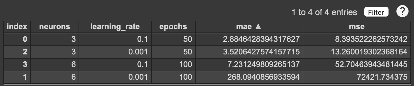
# Show evaluation results in a Pandas DataFrame
import pandas as pd
pd.DataFrame(evaluation_results)
The table below shows that, in this run, the Sequential model with 3 neurons and the Adam optimiser at a learning rate of 0.1 has the lowest MAE and MSE of the four candidates.
Final Thoughts
In this post, I evaluated four regression models with TensorFlow, comparing them with the MAE and MSE error metrics to find the best-performing architecture for the hyperparameters I tried. Model evaluation on a held-out test set is the decisive step that distinguishes a model that generalises from one that has merely memorised its training data. In my experiments, the Sequential model with 3 neurons and an Adam optimiser learning rate of 0.1 produced the lowest MAE and MSE — though which combination wins depends on the random seed and TensorFlow version, so don’t expect to reproduce this exact ranking bit-for-bit.
Regression Model Evaluation FAQ
What is the difference between MAE and MSE in regression?
Mean Absolute Error (MAE) averages the absolute differences between predictions and ground truth, so every error contributes proportionally. Mean Squared Error (MSE) squares each error before averaging, which penalises large outliers far more heavily. Use MAE when all errors matter equally; use MSE when large mistakes are especially costly. Both are computed in TensorFlow with tf.keras.losses.mae and tf.keras.losses.mse (the older functional tf.metrics.mean_absolute_error/mean_squared_error aliases were removed in Keras 3).
How do you evaluate a regression model in TensorFlow?
Call model.evaluate(X_test, y_test) on a held-out test set after training, or compute metrics manually from model.predict(X_test). The test set must not be seen during training; reporting metrics on training data overstates performance. Lower MAE and MSE indicate better predictions.
Why use a separate test set instead of training-set metrics?
Training-set metrics measure memorisation, not generalisation. A model can fit training data almost perfectly while failing on unseen inputs. Splitting the data (here, 80% train / 20% test) and evaluating on the test partition reveals the model’s true predictive performance.
Did you like this post? Please let me know if you have any comments or suggestions.
Python posts that might be interesting for youReferences
Related Reading
Enjoyed this? Get more like it.
Weekly notes on AI tools, Python, and what I'm actually building — plus a free copy of Fantastic AI: The 2026 Toolkit.