
What Is Regression in Machine Learning?
Regression is a supervised machine learning task that predicts a continuous numerical value from one or more input features. Regression is defined in Wikipedia as:
In statistical modeling, regression analysis is a set of statistical processes for estimating the relationships between a dependent variable (often called the ‘outcome’ or ‘response’ variable) and one or more independent variables (often called ‘predictors,’ ‘covariates,’ ‘explanatory variables’ or ‘features’). The most common form of regression analysis is linear regression. One finds the line (or a more complex linear combination) that most closely fits the data according to a specific mathematical criterion.
In simple words, we want to predict a numerical value based on some other numerical values, as described in the TensorFlow Developer Certificate course [1] . In Machine Learning, regression analysis is widely used for prediction and forecasting. For instance, we can use regression models to predict house sale prices. The house price can be modeled regarding the number of bedrooms, bathrooms, or garages. Other applications of regression can be to find out how many people will buy the app, to forecast seasonal sales, and even predict coordinates in an object detection task. In simple words, with regression, we want to find out answers to questions “How many?” and “How much?” [1]
Building a Regression Model in TensorFlow: Three Steps
When we model neural networks in TensorFlow with the Keras Sequential API, we generally follow three steps:
- create a model and define the input, hidden and output layers, number of neurons in each layer;
- compile the model with required loss function, optimiser, evaluation metrics;
- fit the model for finding patterns between features and labels.
In the code below, we create a simple example of a regression model with input features stored in X and output
stored in y. For the demonstration purpose, I did not add much data. Instead, we use quite a small sample size to show
how we can create a regression model and further improve it while adjusting hyperparameters in the model and
compiling or fitting it.
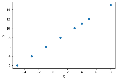
It is also important to mention that linear regression tasks are particularly suitable for a linear trend in the dataset. Our data can be approximated by a line, as shown below. In our example, each y-value can be predicted as X+7.
As we see, the neural network consists just of one hidden layer with one neuron, which is realising the regression functionality.
# Regression example with TensorFlow
import tensorflow as tf
# print(tf.__version__) # 2.7.0

import numpy as np
import matplotlib.pyplot as plt

# Set a random seed for reproducibility
tf.random.set_seed(57)

# Create features
X = np.array([-5., -3., -1., 1., 3., 4., 5., 8.])

# Create labels
y = np.array([2., 4., 6., 8., 10., 11., 12., 15.])

# Turn input and output Numpy arrays into tensors with float32 data type
X = tf.cast(tf.constant(X), dtype=tf.float32)
y = tf.cast(tf.constant(y), dtype=tf.float32)

# Visualise it
plt.scatter(X, y)
plt.xlabel("X")
plt.ylabel("y")

# Expand the X shape for the new version of TensorFlow
X = tf.expand_dims(X, axis=-1)

# Create a Sequential model
model = tf.keras.Sequential([
    tf.keras.layers.Dense(1)
])

# Compile the model with Mean Absolute Error (MAE) loss function and SGD optimiser
model.compile(loss=tf.keras.losses.mae,
              optimizer=tf.keras.optimizers.SGD(),
              metrics=["mae"])

# Fit the model
model.fit(X, y, epochs=5)

# Make predictions
model.predict([[10]])
Epoch 1/5
1/1 [==============================] - 0s 252ms/step - loss: 6.7141 - mae: 6.7141
Epoch 2/5
1/1 [==============================] - 0s 6ms/step - loss: 6.6816 - mae: 6.6816
Epoch 3/5
1/1 [==============================] - 0s 6ms/step - loss: 6.6491 - mae: 6.6491
Epoch 4/5
1/1 [==============================] - 0s 6ms/step - loss: 6.6166 - mae: 6.6166
Epoch 5/5
1/1 [==============================] - 0s 5ms/step - loss: 6.5841 - mae: 6.5841
We have tried to predict unseen data of [10] and observed a significant loss and MAE outputs. The predicted value was [12] instead of the [17] expected.
Improving Regression Model Performance: Hyperparameter Tuning
To improve a regression model, we can apply the following hyperparameter adjustments in any combination, making minor changes one at a time to isolate their effect on model performance [1]:
- adding or removing layers;
- adding the number of hidden neurons;
- changing the activation function;
- changing the optimisation function;
- adjusting the learning rate (potentially, the most critical hyperparameter);
- adding more data;
- increasing the number of epochs;
# Rebuild the model
# Create a Sequential model
model = tf.keras.Sequential([
    tf.keras.layers.Dense(1)
])

# Compile the model with MAE loss function and SGD optimiser
model.compile(loss=tf.keras.losses.mae,
              optimizer=tf.keras.optimizers.Adam(lr=0.1),
              metrics=["mae"])

# Fit the model
model.fit(X, y, epochs=50)

# Make predictions
model.predict([[10]])
/usr/local/lib/python3.7/dist-packages/keras/optimizer_v2/adam.py:105: UserWarning: The `lr` argument is deprecated, use `learning_rate` instead.
  super(Adam, self).__init__(name, **kwargs)
Epoch 1/50
1/1 [==============================] - 0s 261ms/step - loss: 10.2923 - mae: 10.2923
Epoch 2/50
1/1 [==============================] - 0s 9ms/step - loss: 9.9423 - mae: 9.9423
Epoch 3/50
1/1 [==============================] - 0s 7ms/step - loss: 9.5923 - mae: 9.5923
Epoch 4/50
1/1 [==============================] - 0s 5ms/step - loss: 9.2423 - mae: 9.2423
Epoch 5/50
1/1 [==============================] - 0s 5ms/step - loss: 8.8923 - mae: 8.8923
Epoch 6/50
1/1 [==============================] - 0s 5ms/step - loss: 8.5423 - mae: 8.5423
Epoch 7/50
1/1 [==============================] - 0s 8ms/step - loss: 8.2503 - mae: 8.2503
Epoch 8/50
1/1 [==============================] - 0s 5ms/step - loss: 8.0050 - mae: 8.0050
Epoch 9/50
1/1 [==============================] - 0s 6ms/step - loss: 7.7632 - mae: 7.7632
Epoch 10/50
1/1 [==============================] - 0s 5ms/step - loss: 7.5239 - mae: 7.5239
Epoch 11/50
1/1 [==============================] - 0s 5ms/step - loss: 7.2868 - mae: 7.2868
Epoch 12/50
1/1 [==============================] - 0s 6ms/step - loss: 7.0512 - mae: 7.0512
Epoch 13/50
1/1 [==============================] - 0s 5ms/step - loss: 6.8168 - mae: 6.8168
Epoch 14/50
1/1 [==============================] - 0s 6ms/step - loss: 6.5835 - mae: 6.5835
Epoch 15/50
1/1 [==============================] - 0s 4ms/step - loss: 6.3509 - mae: 6.3509
Epoch 16/50
1/1 [==============================] - 0s 7ms/step - loss: 6.1189 - mae: 6.1189
Epoch 17/50
1/1 [==============================] - 0s 8ms/step - loss: 5.8875 - mae: 5.8875
Epoch 18/50
1/1 [==============================] - 0s 6ms/step - loss: 5.6563 - mae: 5.6563
Epoch 19/50
1/1 [==============================] - 0s 8ms/step - loss: 5.4255 - mae: 5.4255
Epoch 20/50
1/1 [==============================] - 0s 7ms/step - loss: 5.1948 - mae: 5.1948
Epoch 21/50
1/1 [==============================] - 0s 5ms/step - loss: 4.9642 - mae: 4.9642
Epoch 22/50
1/1 [==============================] - 0s 11ms/step - loss: 4.7337 - mae: 4.7337
Epoch 23/50
1/1 [==============================] - 0s 7ms/step - loss: 4.5031 - mae: 4.5031
Epoch 24/50
1/1 [==============================] - 0s 11ms/step - loss: 4.2726 - mae: 4.2726
Epoch 25/50
1/1 [==============================] - 0s 7ms/step - loss: 4.0420 - mae: 4.0420
Epoch 26/50
1/1 [==============================] - 0s 6ms/step - loss: 3.8113 - mae: 3.8113
Epoch 27/50
1/1 [==============================] - 0s 10ms/step - loss: 3.5804 - mae: 3.5804
Epoch 28/50
1/1 [==============================] - 0s 9ms/step - loss: 3.4646 - mae: 3.4646
Epoch 29/50
1/1 [==============================] - 0s 5ms/step - loss: 3.4254 - mae: 3.4254
Epoch 30/50
1/1 [==============================] - 0s 4ms/step - loss: 3.3826 - mae: 3.3826
Epoch 31/50
1/1 [==============================] - 0s 5ms/step - loss: 3.3365 - mae: 3.3365
Epoch 32/50
1/1 [==============================] - 0s 8ms/step - loss: 3.3657 - mae: 3.3657
Epoch 33/50
1/1 [==============================] - 0s 7ms/step - loss: 3.3754 - mae: 3.3754
Epoch 34/50
1/1 [==============================] - 0s 7ms/step - loss: 3.3626 - mae: 3.3626
Epoch 35/50
1/1 [==============================] - 0s 9ms/step - loss: 3.3297 - mae: 3.3297
Epoch 36/50
1/1 [==============================] - 0s 6ms/step - loss: 3.2920 - mae: 3.2920
Epoch 37/50
1/1 [==============================] - 0s 10ms/step - loss: 3.2169 - mae: 3.2169
Epoch 38/50
1/1 [==============================] - 0s 9ms/step - loss: 3.1071 - mae: 3.1071
Epoch 39/50
1/1 [==============================] - 0s 9ms/step - loss: 3.0001 - mae: 3.0001
Epoch 40/50
1/1 [==============================] - 0s 5ms/step - loss: 2.8834 - mae: 2.8834
Epoch 41/50
1/1 [==============================] - 0s 8ms/step - loss: 2.7579 - mae: 2.7579
Epoch 42/50
1/1 [==============================] - 0s 6ms/step - loss: 2.6245 - mae: 2.6245
Epoch 43/50
1/1 [==============================] - 0s 8ms/step - loss: 2.5000 - mae: 2.5000
Epoch 44/50
1/1 [==============================] - 0s 7ms/step - loss: 2.4162 - mae: 2.4162
Epoch 45/50
1/1 [==============================] - 0s 7ms/step - loss: 2.3321 - mae: 2.3321
Epoch 46/50
1/1 [==============================] - 0s 6ms/step - loss: 2.2477 - mae: 2.2477
Epoch 47/50
1/1 [==============================] - 0s 4ms/step - loss: 2.1632 - mae: 2.1632
Epoch 48/50
1/1 [==============================] - 0s 6ms/step - loss: 2.0949 - mae: 2.0949
Epoch 49/50
1/1 [==============================] - 0s 7ms/step - loss: 2.0640 - mae: 2.0640
Epoch 50/50
1/1 [==============================] - 0s 6ms/step - loss: 2.0114 - mae: 2.0114
array([[17.117014]], dtype=float32)
We see pretty low loss and MAE values, and the predicted value is close to the trend. We have achieved this by employing the Adam optimiser with learning rate of 0.1 in the model compilation step and increasing the number of epochs while fitting the model.
Evaluating Regression Models with Larger Datasets
Overall, we repeat building and fitting a model with different combinations of hyperparameters. During model training, the model learns patterns from data or finds parameters such as weights. We evaluate the model, tweak the hyperparameters and repeat its building, fitting, and evaluation steps until getting a reasonably good performance.
Overall, we require quite a large dataset to achieve a well-performing machine learning model. The more complex task is, the more data we need. We can start by generating a larger dataset for our regression example.
# Generate a larger data
X = tf.range(-100, 300, 4)
X
<tf.Tensor: shape=(100,), dtype=int32, numpy=
array([-100,  -96,  -92,  -88,  -84,  -80,  -76,  -72,  -68,  -64,  -60,
        -56,  -52,  -48,  -44,  -40,  -36,  -32,  -28,  -24,  -20,  -16,
        -12,   -8,   -4,    0,    4,    8,   12,   16,   20,   24,   28,
         32,   36,   40,   44,   48,   52,   56,   60,   64,   68,   72,
         76,   80,   84,   88,   92,   96,  100,  104,  108,  112,  116,
        120,  124,  128,  132,  136,  140,  144,  148,  152,  156,  160,
        164,  168,  172,  176,  180,  184,  188,  192,  196,  200,  204,
        208,  212,  216,  220,  224,  228,  232,  236,  240,  244,  248,
        252,  256,  260,  264,  268,  272,  276,  280,  284,  288,  292,
        296], dtype=int32)>
# Make labels for the dataset
y = X + 7
y
<tf.Tensor: shape=(100,), dtype=int32, numpy=
array([-93, -89, -85, -81, -77, -73, -69, -65, -61, -57, -53, -49, -45,
       -41, -37, -33, -29, -25, -21, -17, -13,  -9,  -5,  -1,   3,   7,
        11,  15,  19,  23,  27,  31,  35,  39,  43,  47,  51,  55,  59,
        63,  67,  71,  75,  79,  83,  87,  91,  95,  99, 103, 107, 111,
       115, 119, 123, 127, 131, 135, 139, 143, 147, 151, 155, 159, 163,
       167, 171, 175, 179, 183, 187, 191, 195, 199, 203, 207, 211, 215,
       219, 223, 227, 231, 235, 239, 243, 247, 251, 255, 259, 263, 267,
       271, 275, 279, 283, 287, 291, 295, 299, 303], dtype=int32)>
Visualising Regression Data and Model Structure
Data visualisation helps to understand the dataset better. We can also draw training and test performance predictions against the ground truth (or labels). The model’s structure itself can be drawn with the help of TensorFlow’s plot_model functionality.
Train, Validation, and Test Dataset Splits
When we train models, we want to ensure that models do not just learn the data “by heart” but can also work well with unseen data. This property is called model generalisation, which is supported by splitting the dataset into three subsets:
- the training dataset to train our model (70-80% of all data);
- the validation dataset to tune the model (10-15% of data available);
- test dataset to evaluate the model. (10-15% of all data).
For simplicity, we can split our dataset into training and testing sets:
# Split data into train and test sets
X_train = X[:80] # First 80% of the data
y_train = y[:80]
# Test data
X_test = X[80:] # last 20% percent of the data
y_test = y[80:]
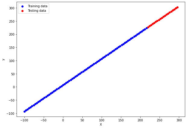
# Visualising the data split into train an test sets
plt.figure(figsize=(10, 7))
# Plot training data in blue
plt.scatter(X_train, y_train, c="b", label="Training data")
# Plot test data in red
plt.scatter(X_test, y_test, c="r", label="Testing data")
plt.legend()
plt.xlabel("X")
plt.ylabel("y")
The figure shows the dataset with training data points in blue and testing data points in red.
We can also perform cross-validation, which I will write in my next post.
Making Predictions with a Trained Regression Model
Let’s create a new model and fit it with the training dataset. The neural network will contain 3 neurons in the first hidden layer and one in the output layer. We keep track of Mean Absolute Error (MAE) and Mean Squared Error (MSE) metrics while using Adam optimiser on the compile step.
# Expanding X to fit the new TensorFlow version requirement
# X = tf.expand_dims(X, axis=-1)

# Create a Sequential model
model = tf.keras.Sequential([
    tf.keras.layers.Dense(3, name="first_layer"),
    tf.keras.layers.Dense(1, name="output_layer")
])


# Compile the model with MAE loss function and SGD optimiser
model.compile(loss=tf.keras.losses.mae,
              optimizer=tf.keras.optimizers.Adam(lr=0.1),
              metrics=["mae", "mse"])

# Fit the model
model.fit(X, y, epochs=50)
/usr/local/lib/python3.7/dist-packages/keras/optimizer_v2/adam.py:105: UserWarning: The `lr` argument is deprecated, use `learning_rate` instead.
  super(Adam, self).__init__(name, **kwargs)
Epoch 1/50
4/4 [==============================] - 0s 3ms/step - loss: 120.9953 - mae: 120.9953 - mse: 23894.6367
Epoch 2/50
4/4 [==============================] - 0s 4ms/step - loss: 37.3695 - mae: 37.3695 - mse: 2743.7510
Epoch 3/50
4/4 [==============================] - 0s 4ms/step - loss: 30.2086 - mae: 30.2086 - mse: 1857.1360
Epoch 4/50
4/4 [==============================] - 0s 3ms/step - loss: 36.0968 - mae: 36.0968 - mse: 2010.0787
Epoch 5/50
4/4 [==============================] - 0s 4ms/step - loss: 22.9426 - mae: 22.9426 - mse: 899.0366
Epoch 6/50
4/4 [==============================] - 0s 5ms/step - loss: 19.2425 - mae: 19.2425 - mse: 539.2803
Epoch 7/50
4/4 [==============================] - 0s 4ms/step - loss: 11.3198 - mae: 11.3198 - mse: 230.8450
Epoch 8/50
4/4 [==============================] - 0s 4ms/step - loss: 11.6120 - mae: 11.6120 - mse: 245.3984
Epoch 9/50
4/4 [==============================] - 0s 4ms/step - loss: 16.8810 - mae: 16.8810 - mse: 422.8721
Epoch 10/50
4/4 [==============================] - 0s 5ms/step - loss: 15.4557 - mae: 15.4557 - mse: 409.4062
Epoch 11/50
4/4 [==============================] - 0s 4ms/step - loss: 9.3804 - mae: 9.3804 - mse: 163.5114
Epoch 12/50
4/4 [==============================] - 0s 4ms/step - loss: 6.3950 - mae: 6.3950 - mse: 63.2417
Epoch 13/50
4/4 [==============================] - 0s 3ms/step - loss: 7.1727 - mae: 7.1727 - mse: 97.3974
Epoch 14/50
4/4 [==============================] - 0s 3ms/step - loss: 4.3348 - mae: 4.3348 - mse: 30.1714
Epoch 15/50
4/4 [==============================] - 0s 3ms/step - loss: 7.2365 - mae: 7.2365 - mse: 97.9294
Epoch 16/50
4/4 [==============================] - 0s 4ms/step - loss: 7.9825 - mae: 7.9825 - mse: 122.1995
Epoch 17/50
4/4 [==============================] - 0s 4ms/step - loss: 7.0333 - mae: 7.0333 - mse: 95.2871
Epoch 18/50
4/4 [==============================] - 0s 3ms/step - loss: 6.7239 - mae: 6.7239 - mse: 74.4304
Epoch 19/50
4/4 [==============================] - 0s 4ms/step - loss: 4.4470 - mae: 4.4470 - mse: 31.7933
Epoch 20/50
4/4 [==============================] - 0s 4ms/step - loss: 1.7557 - mae: 1.7557 - mse: 4.8011
Epoch 21/50
4/4 [==============================] - 0s 5ms/step - loss: 2.2091 - mae: 2.2091 - mse: 7.5242
Epoch 22/50
4/4 [==============================] - 0s 4ms/step - loss: 3.2336 - mae: 3.2336 - mse: 20.6686
Epoch 23/50
4/4 [==============================] - 0s 3ms/step - loss: 6.2744 - mae: 6.2744 - mse: 77.9671
Epoch 24/50
4/4 [==============================] - 0s 4ms/step - loss: 9.0602 - mae: 9.0602 - mse: 135.6305
Epoch 25/50
4/4 [==============================] - 0s 3ms/step - loss: 3.6392 - mae: 3.6392 - mse: 21.3788
Epoch 26/50
4/4 [==============================] - 0s 4ms/step - loss: 1.2313 - mae: 1.2313 - mse: 2.7846
Epoch 27/50
4/4 [==============================] - 0s 3ms/step - loss: 4.6018 - mae: 4.6018 - mse: 35.7042
Epoch 28/50
4/4 [==============================] - 0s 3ms/step - loss: 5.4567 - mae: 5.4567 - mse: 53.5563
Epoch 29/50
4/4 [==============================] - 0s 4ms/step - loss: 3.9640 - mae: 3.9640 - mse: 33.2863
Epoch 30/50
4/4 [==============================] - 0s 3ms/step - loss: 2.6091 - mae: 2.6091 - mse: 13.5995
Epoch 31/50
4/4 [==============================] - 0s 5ms/step - loss: 7.2700 - mae: 7.2700 - mse: 86.4028
Epoch 32/50
4/4 [==============================] - 0s 3ms/step - loss: 10.4771 - mae: 10.4771 - mse: 171.6588
Epoch 33/50
4/4 [==============================] - 0s 3ms/step - loss: 8.3980 - mae: 8.3980 - mse: 161.0003
Epoch 34/50
4/4 [==============================] - 0s 4ms/step - loss: 4.2892 - mae: 4.2892 - mse: 43.4268
Epoch 35/50
4/4 [==============================] - 0s 3ms/step - loss: 1.9115 - mae: 1.9115 - mse: 8.9037
Epoch 36/50
4/4 [==============================] - 0s 3ms/step - loss: 5.1150 - mae: 5.1150 - mse: 46.9002
Epoch 37/50
4/4 [==============================] - 0s 4ms/step - loss: 6.2562 - mae: 6.2562 - mse: 74.0645
Epoch 38/50
4/4 [==============================] - 0s 3ms/step - loss: 3.2418 - mae: 3.2418 - mse: 17.0526
Epoch 39/50
4/4 [==============================] - 0s 5ms/step - loss: 3.0819 - mae: 3.0819 - mse: 18.1384
Epoch 40/50
4/4 [==============================] - 0s 4ms/step - loss: 2.2617 - mae: 2.2617 - mse: 9.4483
Epoch 41/50
4/4 [==============================] - 0s 3ms/step - loss: 4.8202 - mae: 4.8202 - mse: 47.1045
Epoch 42/50
4/4 [==============================] - 0s 4ms/step - loss: 7.5390 - mae: 7.5390 - mse: 125.5217
Epoch 43/50
4/4 [==============================] - 0s 3ms/step - loss: 4.8652 - mae: 4.8652 - mse: 39.2499
Epoch 44/50
4/4 [==============================] - 0s 4ms/step - loss: 4.8499 - mae: 4.8499 - mse: 42.2790
Epoch 45/50
4/4 [==============================] - 0s 4ms/step - loss: 1.0383 - mae: 1.0383 - mse: 3.7415
Epoch 46/50
4/4 [==============================] - 0s 3ms/step - loss: 0.8587 - mae: 0.8587 - mse: 1.4711
Epoch 47/50
4/4 [==============================] - 0s 4ms/step - loss: 1.6601 - mae: 1.6601 - mse: 6.1024
Epoch 48/50
4/4 [==============================] - 0s 3ms/step - loss: 3.7125 - mae: 3.7125 - mse: 30.4232
Epoch 49/50
4/4 [==============================] - 0s 6ms/step - loss: 5.7093 - mae: 5.7093 - mse: 60.4152
Epoch 50/50
4/4 [==============================] - 0s 4ms/step - loss: 5.1068 - mae: 5.1068 - mse: 39.9806
We use plot_model() method to draw the network shown below.
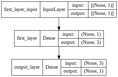
# Import plot_model
from tensorflow.keras.utils import plot_model

plot_model(model, show_shapes=True)
It is helpful to explore how far the model predictions are from the ground truth. We visualise the model predictions against the ground truth in a scatter plot.
# Make some predictions
y_pred = model.predict(X_test)

# Print the predicted and ground truth values
for predicted, truth in zip(y_pred, y_test):
  print("Ground truth:%d    predicted:%f"%(truth.numpy(), predicted[0]))
Ground truth:227    predicted:217.726746
Ground truth:231    predicted:221.557556
Ground truth:235    predicted:225.388351
Ground truth:239    predicted:229.219147
Ground truth:243    predicted:233.049957
Ground truth:247    predicted:236.880753
Ground truth:251    predicted:240.711548
Ground truth:255    predicted:244.542343
Ground truth:259    predicted:248.373154
Ground truth:263    predicted:252.203949
Ground truth:267    predicted:256.034760
Ground truth:271    predicted:259.865570
Ground truth:275    predicted:263.696350
Ground truth:279    predicted:267.527161
Ground truth:283    predicted:271.357971
Ground truth:287    predicted:275.188782
Ground truth:291    predicted:279.019562
Ground truth:295    predicted:282.850372
Ground truth:299    predicted:286.681152
Ground truth:303    predicted:290.511963
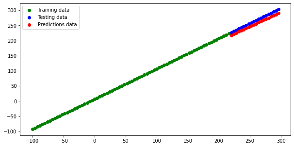
Finally, we create a data plotting function to draw scatter plots of training, testing and predicted datasets.
# A plotting function
def plot_data(train_data=X_train, train_labels=y_train,
                     test_data=X_test, test_labels=y_test, predictions=y_pred):
  plt.figure(figsize=(10, 5))
  # Drawing scatter plots
  plt.scatter(train_data, train_labels, c="g", label="Training data")
  plt.scatter(test_data, test_labels, c="b", label="Testing data")
  plt.scatter(test_data, predictions, c="r", label="Predictions data")
  plt.legend()

plot_data()
The predicted data is below the testing data values, as we see from the plot.
Evaluating Model Predictions with MAE and MSE
We use the model’s evaluate() method with the testing dataset to evaluate the model predictions.
Since we defined the MAE and MSE metrics during the compilation step, we get these values in the result.
# Evaluate the model on the test set
model.evaluate(X_test, y_test)
1/1 [==============================] - 0s 125ms/step - loss: 10.4243 - mae: 10.4243 - mse: 109.5560
[10.424253463745117, 10.424253463745117, 109.55604553222656]
We can also calculate the MAE and MSE having predicted (y_pred) and ground truth labels (y_test).
# Calculate the Mean Absolute Error (MAE) with y_pred and y_test
# Please note that we remove an extra dimension with tf.squeeze
mae = tf.metrics.mean_absolute_error(y_true=y_test, y_pred=tf.squeeze(y_pred))

# Calculate the Mean Square Error (MSE)
mse = tf.metrics.mean_squared_error(y_true=y_test, y_pred=tf.squeeze(y_pred))

print("MAE=%f, MSE=%f"%(mae, mse))
MAE=10.415435, MSE=109.370789
Did you like this post? Please let me know if you have any comments or suggestions.
Python posts that might be interesting for youSummary: Regression Modeling in TensorFlow
A TensorFlow regression model predicts a continuous numerical value through three steps — building a Keras Sequential model, compiling it with a loss function and optimiser, and fitting it to data. This post generated a dataset, split it into training and testing sets, visualised the data and network structure, tuned hyperparameters (Adam optimiser with learning_rate=0.1, 50 epochs), and evaluated predictions with MAE and MSE. In my next post, I cover model evaluation and the widely used cross-validation technique.
For writing this post, I have used the TensorFlow documentation and tutorials at Udemy, TensorFlow Developer Certificate in 2022: Zero to Mastery.
TensorFlow Regression FAQ
How do you build a regression model in TensorFlow?
Follow three steps with the Keras Sequential API: (1) create the model and define its layers with tf.keras.Sequential([tf.keras.layers.Dense(1)]); (2) compile it with a loss function, optimiser, and metrics, e.g. model.compile(loss=tf.keras.losses.mae, optimizer=tf.keras.optimizers.Adam(), metrics=['mae']); (3) fit it to the data with model.fit(X, y, epochs=50).
Which loss function and metric should I use for a TensorFlow regression model?
Use Mean Absolute Error (MAE, tf.keras.losses.mae) or Mean Squared Error (MSE) as the loss for predicting numerical values. Track mae and mse as metrics during compilation so model.evaluate() returns them for the test set. MAE reports the average absolute prediction error in the target’s units; MSE penalises larger errors more heavily.
How can I improve a regression model’s predictions in TensorFlow?
Adjust hyperparameters one at a time: add or remove layers, change the number of hidden neurons, change the activation or optimisation function, tune the learning rate (often the most critical hyperparameter), add more data, or increase the number of epochs. In this post, switching to the Adam optimiser with learning_rate=0.1 and raising epochs from 5 to 50 moved the prediction for input 10 from 12 to 17.1, close to the expected 17.
What does the warning ‘The lr argument is deprecated, use learning_rate instead’ mean?
TensorFlow/Keras renamed the optimiser argument lr to learning_rate. Replace tf.keras.optimizers.Adam(lr=0.1) with tf.keras.optimizers.Adam(learning_rate=0.1) to silence the UserWarning and stay compatible with current Keras versions.
Bibliography
Related Reading
Enjoyed this? Get more like it.
Weekly notes on AI tools, Python, and what I'm actually building — plus a free copy of Fantastic AI: The 2026 Toolkit.