Introduction

In machine learning, it’s crucial to evaluate the performance of our models accurately and reliably. One of the most common methods for achieving this is cross-validation. Cross-validation helps us assess how well our model will generalise to unseen data and avoid overfitting.

In this post, we will explore the concept of generalisation and explore various cross-validation techniques using the Titanic dataset and Ihe Daily Minimum Temperatures dataset (for time series splits). We’ll also discuss implementing these techniques in scikit-learn.

Prerequisites

Before we begin, ensure you have the following Python libraries installed:

• scikit-learn (for machine learning)
• pandas (for data manipulation)
• numpy (for numerical operations)
• matplotlib (for visualisation)

You can install them using pip:

pip install scikit-learn pandas numpy matplotlib

Additionally, download the Titanic dataset from Kaggle and place it in your working directory.

You can also get the Titanic dataset from my GitHub repository directly to your Colab as follows:

import pandas as pd

url = 'https://raw.githubusercontent.com/edaehn/python_tutorials/main/titanic/train.csv'
titanic_df = pd.read_csv(url)
titanic_df.head()

I suggest using Colab, which has Gemini AI working "under the hood", and you can ask it to write or explain code. It is AWESOME!

Please note that all the code will be uploaded into the python_tutorials in the following days.

Understanding Generalisation

Generalisation refers to how well a machine learning model performs on new, unseen data. A model that generalises well can accurately predict outcomes for data it hasn’t encountered during training. Generalisation is essential to ensure that your model isn’t just memorising the training data (overfitting) but learning meaningful patterns that apply broadly.

What is Cross-Validation?

Cross-validation is a technique for assessing the performance of a machine-learning model. Instead of using a single train-test split, cross-validation involves dividing the dataset into multiple subsets and repeatedly training and testing the model on different combinations of these subsets. This provides a more robust evaluation of model performance.

The Main Purpose of Cross-Validation

The primary purposes of cross-validation are to:

1. Estimate how well a model will generalise to new, unseen data
2. Detect and prevent overfitting by evaluating the model’s performance on various data subsets
3. Make efficient use of limited data by utilising it for both training and validation
4. Provide confidence intervals for performance metrics

Cross-validation Tradeoff

The cross-validation tradeoff refers to the balance between model complexity and the ability to generalise to unseen data when using cross-validation techniques. It’s an essential consideration when applying cross-validation methods in machine learning. The tradeoff can be summarized as follows:

1. High Model Complexity:
   • Pros: A complex model may perform exceptionally well on the training data.
   • Cons: It’s more prone to overfitting, which may not generalise well to unseen data.
2. Low Model Complexity:
   • Pros: A simpler model is less likely to overfit the training data.
   • Cons: It may not capture complex patterns in the data and could underfit, resulting in poor predictive performance.

If you did not read my post Bias-Variance Challenge, I suggest you read it before getting started. In that post, we covered the model fitting process and struck the right balance to achieve model generalisation. We also calculated bias and variance, which might be helpful.

The bias-variance dilemma graph (previously shared in post Bias-Variance Challenge) is shown below.

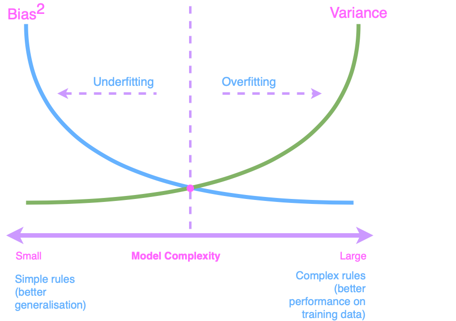
Cross-validation techniques, such as K-Fold, Stratified K-Fold, and Leave-One-Out, help you balance these extremes. By dividing your data into multiple subsets and systematically training and testing your model, you can assess how different levels of model complexity affect generalisation.

The goal is to find the optimal model complexity that minimises overfitting while still capturing meaningful patterns in the data. This involves iteratively adjusting hyperparameters, feature selection, or using different models, and evaluating their performance during cross-validation. The tradeoff aims to ensure your model is both interpretable and predictive, making it a valuable tool in real-world applications.

Learning Curves

Learning curves are graphical representations that illustrate how an estimator’s performance evolves as the training dataset’s size varies. They are essential tools for assessing the impact of additional training data on an estimator’s performance and for diagnosing whether the model is affected by high bias or high variance.

Learning curves consist of two critical components:

• Training scores: Measure how well the model fits the training data
• Validation scores: Indicate how well the model generalizes to unseen data

The primary purposes of learning curves are:

1. Estimating the Impact of Training Data Size: We can observe how performance changes with more data by plotting the training and validation scores against the number of training samples. If both scores plateau as the dataset size increases, acquiring more data may not significantly improve performance.

2. Detecting Bias and Variance Issues:

   • If both training and validation scores converge to a low value, the model likely suffers from high bias (underfitting)
   • If there’s a significant gap between high training scores and low validation scores, the model likely suffers from high variance (overfitting)

Here’s an example of implementing learning curves with a Random Forest classifier on the Titanic dataset:

import numpy as np
import pandas as pd
import matplotlib.pyplot as plt
from sklearn.ensemble import RandomForestClassifier
from sklearn.model_selection import learning_curve
from sklearn.model_selection import train_test_split
from sklearn.preprocessing import StandardScaler, OneHotEncoder
from sklearn.compose import ColumnTransformer
from sklearn.pipeline import Pipeline
from sklearn.impute import SimpleImputer

# Load the Titanic dataset
# Note: Replace with your path to the Titanic dataset
titanic = pd.read_csv('titanic/train.csv')

# Basic preprocessing
# Select relevant features
features = ['Pclass', 'Sex', 'Age', 'SibSp', 'Parch', 'Fare', 'Embarked']
X = titanic[features]
y = titanic['Survived']

# Define preprocessing for numerical and categorical features
numerical_features = ['Age', 'SibSp', 'Parch', 'Fare']
categorical_features = ['Pclass', 'Sex', 'Embarked']

numerical_transformer = Pipeline(steps=[
    ('imputer', SimpleImputer(strategy='median')),
    ('scaler', StandardScaler())
])

categorical_transformer = Pipeline(steps=[
    ('imputer', SimpleImputer(strategy='constant', fill_value='missing')),
    ('onehot', OneHotEncoder(handle_unknown='ignore'))
])

preprocessor = ColumnTransformer(
    transformers=[
        ('num', numerical_transformer, numerical_features),
        ('cat', categorical_transformer, categorical_features)
    ])

# Create a pipeline with preprocessing and Random Forest classifier
rf_pipeline = Pipeline(steps=[
    ('preprocessor', preprocessor),
    ('classifier', RandomForestClassifier(n_estimators=100, random_state=42))
])

# Calculate learning curves
train_sizes, train_scores, test_scores = learning_curve(
    rf_pipeline, X, y, cv=5, 
    train_sizes=np.linspace(0.1, 1.0, 10),
    scoring='accuracy',
    random_state=42
)

# Calculate the mean and standard deviation of the training and test scores
train_mean = np.mean(train_scores, axis=1)
train_std = np.std(train_scores, axis=1)
test_mean = np.mean(test_scores, axis=1)
test_std = np.std(test_scores, axis=1)

# Plot the learning curves
plt.figure(figsize=(10, 6))
plt.title("Learning Curves (Random Forest)")
plt.xlabel("Training Examples")
plt.ylabel("Accuracy")
plt.grid()

plt.fill_between(train_sizes, train_mean - train_std, train_mean + train_std, alpha=0.1, color="blue")
plt.fill_between(train_sizes, test_mean - test_std, test_mean + test_std, alpha=0.1, color="red")
plt.plot(train_sizes, train_mean, marker="o", markersize=5, color="blue", label="Training Accuracy")
plt.plot(train_sizes, test_mean, marker="o", markersize=5, color="red", label="Validation Accuracy")

plt.legend(loc="best")
plt.tight_layout()
plt.show()

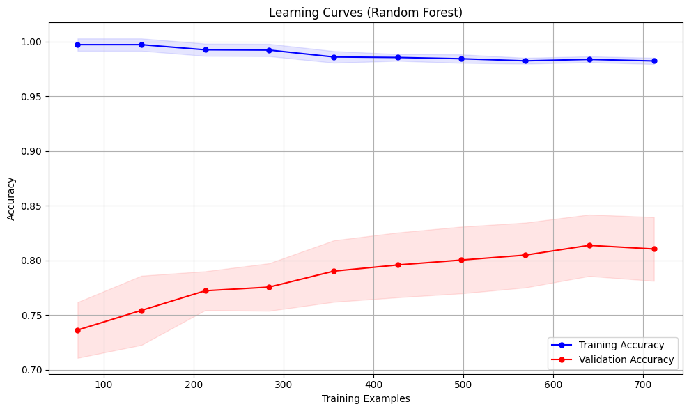
The code above creates a proper preprocessing pipeline, handles missing values, and plots learning curves to visualize how the model’s performance changes with increasing training data size.

I am mesmerised by the ease of drawing simple graphs with AI nowadays. I still remember my PhD research and coding experience when I had to code everything from scratch without AI! I expect now that researchers and everyone can spend their time more wisely! :)

Different Cross-Validation Techniques

Hold-Out Cross-Validation

Hold-out is the simplest cross-validation method. It involves splitting the dataset into a training set and a validation set. Here’s an example using scikit-learn:

from sklearn.model_selection import train_test_split

X_train, X_val, y_train, y_val = train_test_split(X, y, test_size=0.2, random_state=42)

This code randomly splits your dataset into two parts: one for training your machine learning model and another, held back, for testing how well the model generalises to unseen data. This helps to prevent overfitting, where your model performs well on the training data but poorly on new data.

While simple, this method’s main limitation is that the evaluation depends heavily on which data points are in the training and validation sets.

K-Fold Cross-Validation

K-Fold divides the dataset into ‘k’ equal-sized subsets (folds). The model is trained ‘k’ times, each using a different fold as the validation set and the remaining folds as the training set.

from sklearn.model_selection import KFold
from sklearn.metrics import accuracy_score
import numpy as np

kf = KFold(n_splits=5, shuffle=True, random_state=42)
scores = []

for train_index, val_index in kf.split(X):
    X_train, X_val = X.iloc[train_index], X.iloc[val_index]
    y_train, y_val = y.iloc[train_index], y.iloc[val_index]
    
    # Train your model
    rf_pipeline.fit(X_train, y_train)
    
    # Evaluate on validation set
    y_pred = rf_pipeline.predict(X_val)
    score = accuracy_score(y_val, y_pred)
    scores.append(score)

print(f"Cross-validation scores: {scores}")
print(f"Mean accuracy: {np.mean(scores)}")
print(f"Standard deviation: {np.std(scores)}")

Cross-validation scores: [0.8100558659217877, 0.7808988764044944, 0.8314606741573034, 0.8089887640449438, 0.8370786516853933]
Mean accuracy: 0.8136965664427847
Standard deviation: 0.019866514584768555

Leave-One-Out (LOO) Cross-Validation

LOO creates ‘n’ folds, where ‘n’ is the number of data points. In each iteration, one data point is used for validation, and all others are used for training. It’s computationally expensive but provides an unbiased model performance estimate.

from sklearn.model_selection import LeaveOneOut
from sklearn.metrics import accuracy_score

loo = LeaveOneOut()
scores = []

for train_index, val_index in loo.split(X):
    X_train, X_val = X.iloc[train_index], X.iloc[val_index]
    y_train, y_val = y.iloc[train_index], y.iloc[val_index]
    
    # Train your model
    rf_pipeline.fit(X_train, y_train)
    
    # Evaluate on the single validation example
    y_pred = rf_pipeline.predict(X_val)
    score = accuracy_score(y_val, y_pred)
    scores.append(score)

print(f"Mean accuracy: {np.mean(scores)}")

Mean accuracy: 0.8215488215488216

Stratified K-Fold Cross-Validation

Stratified K-Fold maintains the class distribution in each fold, making it suitable for imbalanced datasets where certain classes appear much less frequently than others.

from sklearn.model_selection import StratifiedKFold
from sklearn.metrics import accuracy_score, classification_report

skf = StratifiedKFold(n_splits=5, shuffle=True, random_state=42)
scores = []

for train_index, val_index in skf.split(X, y):
    X_train, X_val = X.iloc[train_index], X.iloc[val_index]
    y_train, y_val = y.iloc[train_index], y.iloc[val_index]
    
    # Train your model
    rf_pipeline.fit(X_train, y_train)
    
    # Evaluate on validation set
    y_pred = rf_pipeline.predict(X_val)
    score = accuracy_score(y_val, y_pred)
    scores.append(score)
    
    # For the last fold, print detailed classification report
    if len(scores) == 5:
        print(classification_report(y_val, y_pred))

print(f"Cross-validation scores: {scores}")
print(f"Mean accuracy: {np.mean(scores)}")

precision    recall  f1-score   support

           0       0.86      0.91      0.88       109
           1       0.84      0.77      0.80        69

    accuracy                           0.85       178
   macro avg       0.85      0.84      0.84       178
weighted avg       0.85      0.85      0.85       178

Cross-validation scores: [0.8379888268156425, 0.7921348314606742, 0.7808988764044944, 0.8202247191011236, 0.8539325842696629]
Mean accuracy: 0.8170359676103196

Repeated K-Fold Cross-Validation

Repeated K-Fold performs K-Fold multiple times with different random splits, providing a more robust estimate of model performance by reducing the variance of the evaluation.

from sklearn.model_selection import RepeatedKFold
from sklearn.metrics import accuracy_score

rkf = RepeatedKFold(n_splits=5, n_repeats=3, random_state=42)
scores = []

for train_index, val_index in rkf.split(X):
    X_train, X_val = X.iloc[train_index], X.iloc[val_index]
    y_train, y_val = y.iloc[train_index], y.iloc[val_index]
    
    # Train your model
    rf_pipeline.fit(X_train, y_train)
    
    # Evaluate on validation set
    y_pred = rf_pipeline.predict(X_val)
    score = accuracy_score(y_val, y_pred)
    scores.append(score)

print(f"Mean accuracy: {np.mean(scores)}")
print(f"Standard deviation: {np.std(scores)}")

Mean accuracy: 0.8103236875693095
Standard deviation: 0.0191686368620614

Time Series Cross-Validation

Time Series Cross-Validation is specifically designed for time series data. It ensures that training data comes before validation data in chronological order, respecting the temporal nature of the data.

Surely, the Titanic dataset is not ideal for this task. I recommend searching other publicly available datasets and reading the docs TimeSeriesSplit.

A simple and commonly used example is the Daily Minimum Temperatures dataset, which tracks the daily minimum air temperatures in Melbourne, Australia, from 1981 to 1990. It’s a univariate time series but is perfectly suitable for demonstrating time-series splits. You can download it (as a CSV file) directly from a public GitHub repo, for instance:

https://raw.githubusercontent.com/jbrownlee/Datasets/master/daily-min-temperatures.csv

Below is a minimal working example that shows how you might load this dataset into a pandas DataFrame, use scikit-learn’s TimeSeriesSplit for cross-validation, and evaluate a model’s Mean Squared Error on each split.

from sklearn.model_selection import TimeSeriesSplit
from sklearn.metrics import mean_squared_error
from sklearn.ensemble import RandomForestRegressor
from sklearn.preprocessing import StandardScaler

# 1. Load the dataset
url = "https://raw.githubusercontent.com/jbrownlee/Datasets/master/daily-min-temperatures.csv"
df = pd.read_csv(url, parse_dates=["Date"])  # parse Date column as datetime
df = df.sort_values("Date")                  # ensure chronological order

# Just to illustrate, X can be additional features derived from Temp
# For this toy example, let's just pretend 'Temp' itself is our only feature
df["Temp_lag1"] = df["Temp"].shift(1)  # example lag feature
df["Temp_lag2"] = df["Temp"].shift(2)  # another lag feature
df.dropna(inplace=True)                # remove first rows with NaN lags

# Features (X) and target (y)
X = df[["Temp", "Temp_lag1", "Temp_lag2"]]
y = df["Temp"]

# 2. Create a simple pipeline with scaling and a random forest regressor
rf_pipeline = Pipeline([
    ("scaler", StandardScaler()),
    ("rf", RandomForestRegressor())
])

# 3. Set up TimeSeriesSplit
tscv = TimeSeriesSplit(n_splits=5)
scores = []

for train_index, val_index in tscv.split(X):
    X_train, X_val = X.iloc[train_index], X.iloc[val_index]
    y_train, y_val = y.iloc[train_index], y.iloc[val_index]
    
    # Train the model
    rf_pipeline.fit(X_train, y_train)
    
    # Predict on the validation set
    y_pred = rf_pipeline.predict(X_val)
    
    # Compute MSE
    score = mean_squared_error(y_val, y_pred)
    scores.append(score)

print(f"Time Series CV MSE scores: {scores}")
print(f"Mean MSE: {np.mean(scores)}")

Time Series CV MSE scores: [0.001360139802631584, 0.0026464062499999908, 0.0009373042763157611, 0.0051862796052638575, 0.0012855899506579217]
Mean MSE: 0.002283143976973823

Please note:

1. Chronological Order: Because TimeSeriesSplit assumes that earlier indices come before later indices, ensure your data is sorted by date (as shown above).
2. Feature Engineering: In a real scenario, you’d often create additional lagged features, rolling means, or domain-specific features to help the model learn temporal patterns.
3. Public Dataset: This particular CSV is small, univariate, and very common in time series tutorials. You can quickly adapt the same approach to larger or more complex time series datasets.

Using GPU in Colab with scikit-learn

For faster processing, I recommend using GPU when possible and it makes sense. Remember, not all algorithms work well with parallel processing. I promise to write a post about GPU soon.

While scikit-learn was traditionally CPU-focused, recent versions support GPU acceleration for specific algorithms through the scikit-learn-intelex extension.

Google Colab provides free access to GPUs, making it an excellent platform for accelerated machine learning experiments.

1. First, ensure you have GPU enabled in your Colab notebook:
   • Go to Runtime > Change runtime type
   • Select GPU from the hardware accelerator dropdown
   • Click Save
2. Install scikit-learn-intelex:

!pip install scikit-learn-intelex

1. Enable GPU acceleration:

from sklearnex import patch_sklearn
patch_sklearn()

# Now import and use scikit-learn as usual
import sklearn
print(f"scikit-learn version: {sklearn.__version__}")

If everything goes well, you will get the Intel(R) confirmation as follows:

scikit-learn version: 1.6.1
Intel(R) Extension for Scikit-learn* enabled (https://github.com/uxlfoundation/scikit-learn-intelex)

Future reading

To understand how the indeces are selected for each cross-validation approach, I recommend reading the scikit-learn docs Visualizing cross-validation behavior in scikit-learn. You can actually observe how the data is sampled in colourful graphs.

Best Practices

Cross-validation best practices ensure reliable model evaluation and parameter optimisation, improving predictive performance while considering dataset complexities and computational resources.

The primary best practices for Cross-Validation follow:

1. Select the appropriate cross-validation method for your data.
2. Shuffle your data before splitting to ensure randomness.
3. Use stratified techniques for imbalanced datasets to maintain class distribution.
4. Perform consistent data preprocessing across all folds to avoid data leakage.
5. Use nested cross-validation for hyperparameter tuning.
6. Experiment with different models to identify the best performer.
7. Apply feature selection within each fold to prevent leakage.
8. Choose a suitable evaluation metric (e.g., accuracy, F1-score, ROC-AUC).
9. Handle missing data uniformly across all folds.
10. Understand the limitations of cross-validation and tailor your approach to your problem specifics.

Conclusion

This post provided a comprehensive overview of cross-validation techniques and how to apply them using the Titanic dataset. By following best practices and experimenting with different cross-validation methods, you can build more robust and generalisable machine-learning models. Good luck!

References

1. Bias-Variance Challenge post
2. Bias-Variance Dilemma image
3. Learning Curves example image
4. Titanic dataset from Kaggle
5. Titanic CSV from GitHub
6. GitHub repo (python_tutorials)
7. Daily Minimum Temperatures dataset
8. TimeSeriesSplit in scikit-learn docs
9. Visualizing cross-validation splits in scikit-learn
10. Scikit-Learn Cross-Validation docs