Introduction: The Bias-Variance Tradeoff in Machine Learning

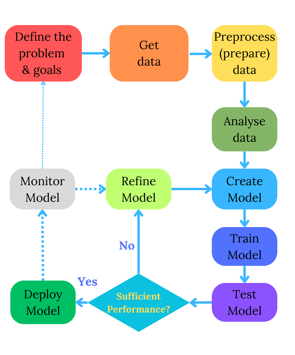
In machine learning, we usually start from a simple baseline model and progressively adjust its complexity until we reach that spot with the best model performance. We play with the model to fine-tune its parameters and complexity in an iterative process described in my previous post, the Machine Learning Process, wherein I have posted this diagram.

We want our Machine Learning (ML) model to solve a particular problem, for instance, detecting spam in e-mail messages.

The model should be well-trained, however, generalisable to new data when new spam messages not existing in the training dataset are received. In short, the model has to be well-fitted.

ML models should be resilient to noisy data, work well on unseen data, and help make unbiased decisions. We want to achieve an optimal variance to make generalisable models work well with new data.

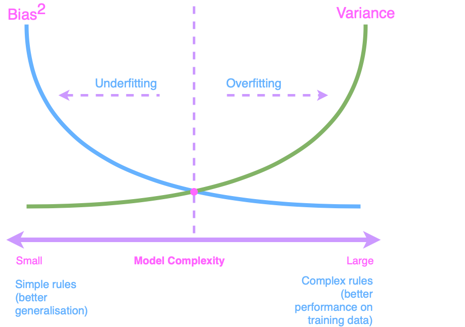
How can we do this? The bias-variance tradeoff is the balance between a model that is too simple (high bias, underfitting) and one that is too complex (high variance, overfitting); the goal is the complexity that minimises total error on unseen data. Let’s detail the most essential machine learning concepts, particularly the bias-variance challenge.

Bias, Variance, and Irreducible Error

Different machine learning algorithms seek to minimise the chosen loss function during training. The algorithm aims to find the model parameters (coefficients or weights) that minimise the error on the training data. Minimising this error helps ensure the model generalises well to unseen data and makes accurate predictions or classifications.

In general, algorithmic error is typically decomposed into three fundamental components, as formalised in The Elements of Statistical Learning (Hastie, Tibshirani & Friedman):

• Bias squared (Bias^2)
• Variance (Variance)
• Irreducible error

Error = Bias^2 + Variance + Irreducible Error

Irreducible error, also known as irreducible uncertainty or irreducible noise, is a component of the total error in a predictive model that cannot be reduced or eliminated by improving the model itself. It represents the inherent unpredictability and randomness in the data or the underlying process being modelled. This error source is considered “irreducible” because it is beyond the control of the model, and no matter how complex or sophisticated the model is, it cannot account for or reduce this source of error.

Irreducible error arises from various factors, including:

1. Inherent Data Variability: Data collected from the real world often contains inherent noise and randomness. Even with a perfect model, there will always be a level of unpredictability in the data.

2. Measurement Error: Data may be subject to measurement errors, inaccuracies, or imprecisions, which introduce noise and contribute to the irreducible error.

3. Unaccounted Variables: There may be unobserved or unmeasured variables that influence the outcome but are not included in the model, leading to unpredictability.

4. Random Events: Some processes, particularly in fields like finance or complex natural systems, are influenced by random events that cannot be modelled or predicted accurately.

The presence of irreducible error is an essential concept in statistics and machine learning. It emphasises that there is a limit to how well a model can perform, as some level of error will always be present due to the intrinsic unpredictability in the data.

Modellers must focus on reducing bias and variance (the reducible components of error) while acknowledging and accepting the existence of irreducible errors in their predictions and analyses.

Let’s define bias and variance concepts.

Bias and variance in detail, the bias-variance challenge and the Python code follow below.

Bias–variance challenge

🔒 Subscribe to keep reading.

Striking the Right Balance

🔒 Subscribe to keep reading.

Computing Bias and Variance in Python with scikit-learn

🔒 Subscribe to keep reading.

Conclusion: Finding the Bias-Variance Sweet Spot

🔒 Subscribe to keep reading.

References

🔒 Subscribe to keep reading.