
Comparing Machine Learning Models on the Titanic Dataset: Introduction
In my “Data exploration and analysis with Python Pandas” post, I described how to use Pandas Python library to analyse, explore and visualise the Titanic dataset. As promised, I will perform Machine Learning tests using this data. I will follow the general steps that it is good to start with when performing ML experiments. I will briefly explain the main ideas of how to start with ML while coding and testing several classification models for predicting the survival of Titanic passengers. I will use Logistic Regression, Decision Tree and Random Forest from Python’s library scikit-learn and a Neural Network created with TensorFlow. That will be a breeze!
What is Machine Learning?
Machine learning is a part of AI and is often performed in the data analysis. Machine Learning can be used for various tasks, such as classification, regression, clustering, and natural language processing. Today we cannot imagine our lives without automatic grammar checks such as those provided by Grammarly and its friends, intelligent chatbots such as chatGPT that are good in poetry, language translators, virtual assistants like Siri, DALL-E creating fantastic images, robots doing high-precision manufacture and self-driving cars, which I did not have a chance to travel yet :)
Machine learning is a branch of artificial intelligence that teaches computers to learn patterns from data without being explicitly programmed. It involves using algorithms to analyse data, learn from it, and make predictions or decisions without human intervention. We can imagine that the ML program is a black box accepting our data, crunching it, and finally giving the result, for instance, recognising a person given a photo.
We need loads of data to train our magic ML black boxes. However, we can also use relatively small datasets. It all depends on what we are doing and how helpful our data elements (called “features”) are for solving our problems. For instance, in my bird species detection tests, I have used quite a large dataset and still needed to build on top of the pre-trained model to achieve reasonable results. Interested? You can read about transfer learning, data augmentation and experimental setup with TensorFlow in my post “TensorFlow: Transfer Learning (Fine-Tuning) in Image Classification” later.
However, that post is a bit challenging to start. We should begin with a simpler task, everyone learning ML knows about the Titanic dataset, which is as famous as George Clooney for ML guys :) No joke, I like coffee and good movies too!
The Titanic dataset, while relatively small, contains a good amount of information, and it’s considered an excellent dataset to start learning ML. It’s often used as a beginner’s dataset for classification and feature engineering tasks because of its simplicity, size and the fact that it’s publicly available. However, depending on the complexity of the model and the problem you are trying to solve, more is needed for more advanced or complex applications. In short, machine learning is a specific technique that is used in data analysis, but not all data analysis tasks require ML.
ML techniques are employed to create intelligent AI systems, which we can make ourselves when we know how. It all sounds exciting. We must learn some math and stats, how to use existing libraries, and coding. Knowing which technique is appropriate and for what task, and how the algorithms behind ML techniques work would be beneficial. There is plenty to learn, but we can start in baby steps by gradually learning everything we like to know.
Supervised Machine Learning
In our experiments, we will predict the survival of Titanic passengers. If we look at our dataset, we can observe that each row in our table contains the “Survived” column, which is a “label” or the target variable we want to predict. We can assume that other columns or variables, such as “Pclass”, “Sex”, “Age” and “Fare” might help predict passenger survival. We have yet to be entirely sure, and we need to try.
We can train several ML models that will learn from the dataset provided with labels. So we require that the data is labelled, and this is why it is called “supervised”. There are also unsupervised, semi-supervised, reinforcement learning techniques, but Supervised Machine Learning is the way to start, at least, in this post :)
titanic_df.head()
| index | PassengerId | Survived | Pclass | Name | Sex | Age | SibSp | Parch | Ticket | Fare | Cabin | Embarked |
|---|---|---|---|---|---|---|---|---|---|---|---|---|
| 0 | 1 | 0 | 3 | Braund, Mr. Owen Harris | male | 22.0 | 1 | 0 | A/5 21171 | 7.25 | NaN | S |
| 1 | 2 | 1 | 1 | Cumings, Mrs. John Bradley (Florence Briggs Thayer) | female | 38.0 | 1 | 0 | PC 17599 | 71.2833 | C85 | C |
| 2 | 3 | 1 | 3 | Heikkinen, Miss. Laina | female | 26.0 | 0 | 0 | STON/O2. 3101282 | 7.925 | NaN | S |
| 3 | 4 | 1 | 1 | Futrelle, Mrs. Jacques Heath (Lily May Peel) | female | 35.0 | 1 | 0 | 113803 | 53.1 | C123 | S |
| 4 | 5 | 0 | 3 | Allen, Mr. William Henry | male | 35.0 | 0 | 0 | 373450 | 8.05 | NaN | S |
We start with the most commonly used supervised learning algorithms performing well. They can be used as benchmarks for building complex systems and can even be sufficient in some applications.
Machine Learning Techniques to Start
In this post, we will try out the following Supervised ML algorithms. We will use the same setup and compare their accuracy. We will predict passenger survival, which is our target label. Titanic passenger attributes (e.g. age, gender, class) will be our input features.
-
Logistic Regression, a supervised learning algorithm that can be used to predict a binary outcome, is what we have. Survived is marked as “1”, and died marked as “0” in our dataset.
-
Decision tree is a supervised learning algorithm that can predict a categorical or continuous outcome. Decision trees work well out-of-box.
-
Random forest is an ensemble learning algorithm (we can also call it supervised, we use the labelled data for building the forest out of trees, as we will see below) that combines the predictions of multiple decision trees to improve the model’s overall accuracy.
-
Neural network is a supervised learning algorithm that can be used to predict a categorical or continuous outcome.
We will use an awesome Python’s library scikit-learn and TensorFlow, the popular open-source machine-learning library developed by Google, to implement and train these machine-learning models in Python.
Machine Learning Steps
The general steps to do ML experiments are:
- Define the problem and determine the goals of the model. That we know - we want to predict the survival of Titanic passengers.
- Collect and preprocess the data. We will use the Titanic dataset saved in a CSV file, load it to Pandas dataframe (read my handy post “Data exploration and analysis with Python Pandas”), preprocess the data in s shape we need.
- Split the data into training and testing sets. That will be useful to test the accuracy of our ML models on unseen data.
- Choose an appropriate algorithm and train the model on the training data. That we already chosen, the Logistic Regression, Decision tree, Random forest, and possibly Neural network should work well for our classification task.
- Evaluate the model’s performance on the testing data. We will use an accuracy metric to measure model performance and compare the selected techniques.
- Fine-tune the model and repeat steps 4 and 5 until satisfactory performance is achieved. This is done in practice, and we will do it in one of my posts about the Titanic dataset. If you are impatient, you can check my oldest post TensorFlow: Transfer Learning (Fine-Tuning) in Image Classification, which is however about working with the image data, and slightly more complicated.
- Use the model to make predictions on new data. That is easy, and we will use the predict() method using trained models.
Installing the libraries
We will use Pandas, Sckikit-learn and TensorFlow. I recommend using Google Colab, which already has all these Python libraries installed. You can connect your Google Drive to store the notebooks and data.
Alternatively, use “pip install libname” for installing Pandas, TensorFlow and Sckikit-learn libraries.
# Upgrade pip
pip install --upgrade pip

# Install the libraries or use -U flag for their upgrade
pip install pandas
pip install -U scikit-learn
pip install tensorflow
Data preprocessing with Pandas
As I have described in my post “Data exploration and analysis with Python Pandas”](https://daehnhardt.com/blog/2023/01/20/pandas-tutorial-with-titanic-dataset/), the Pandas library in Python providing several useful functions for preprocessing data, including manipulating and cleaning data stored in a DataFrame. When working with the Titanic dataset, there are several steps you can take to preprocess the data before building ML models to predict passenger survival.
In this section, I will recite several useful ways to process data. You can skip this section and go to the “Splitting the dataset” section if you know a bit about Pandas and cannot wait. I advise you to read through so that you can keep an eye on the possibilities of what you can do with your data, Titanic or, perhaps, another project.
Import Pandas
Naturally, we need to import libraries to use them.
import pandas as pd
Load the dataset into a DataFrame
url = 'https://raw.githubusercontent.com/edaehn/python_tutorials/main/titanic/train.csv'
titanic_df = pd.read_csv(url)
titanic_df.head()
| index | PassengerId | Survived | Pclass | Name | Sex | Age | SibSp | Parch | Ticket | Fare | Cabin | Embarked |
|---|---|---|---|---|---|---|---|---|---|---|---|---|
| 0 | 1 | 0 | 3 | Braund, Mr. Owen Harris | male | 22.0 | 1 | 0 | A/5 21171 | 7.25 | NaN | S |
| 1 | 2 | 1 | 1 | Cumings, Mrs. John Bradley (Florence Briggs Thayer) | female | 38.0 | 1 | 0 | PC 17599 | 71.2833 | C85 | C |
| 2 | 3 | 1 | 3 | Heikkinen, Miss. Laina | female | 26.0 | 0 | 0 | STON/O2. 3101282 | 7.925 | NaN | S |
| 3 | 4 | 1 | 1 | Futrelle, Mrs. Jacques Heath (Lily May Peel) | female | 35.0 | 1 | 0 | 113803 | 53.1 | C123 | S |
| 4 | 5 | 0 | 3 | Allen, Mr. William Henry | male | 35.0 | 0 | 0 | 373450 | 8.05 | NaN | S |
Use the info() function to get a summary of information about our data, columns, their data types and memory usage.
titanic_df.info()
<class 'pandas.core.frame.DataFrame'>
RangeIndex: 891 entries, 0 to 890
Data columns (total 12 columns):
 #   Column       Non-Null Count  Dtype
---  ------       --------------  -----
 0   PassengerId  891 non-null    int64
 1   Survived     891 non-null    int64
 2   Pclass       891 non-null    int64
 3   Name         891 non-null    object
 4   Sex          891 non-null    object
 5   Age          714 non-null    float64
 6   SibSp        891 non-null    int64
 7   Parch        891 non-null    int64
 8   Ticket       891 non-null    object
 9   Fare         891 non-null    float64
 10  Cabin        204 non-null    object
 11  Embarked     889 non-null    object
dtypes: float64(2), int64(5), object(5)
memory usage: 83.7+ KB
Handle missing values
You can use the fillna() function to replace missing values in the dataset with a specific value or interpolate the missing values using methods such as mean or median. Note that we have created a new variable, “df_preprocesed”, for further data preprocessing.
df_preprocesed = titanic_df.fillna(titanic_df.mean())
df_preprocesed.head()
| index | PassengerId | Survived | Pclass | Name | Sex | Age | SibSp | Parch | Ticket | Fare | Cabin | Embarked |
|---|---|---|---|---|---|---|---|---|---|---|---|---|
| 0 | 1 | 0 | 3 | Braund, Mr. Owen Harris | male | 22.0 | 1 | 0 | A/5 21171 | 7.25 | NaN | S |
| 1 | 2 | 1 | 1 | Cumings, Mrs. John Bradley (Florence Briggs Thayer) | female | 38.0 | 1 | 0 | PC 17599 | 71.2833 | C85 | C |
| 2 | 3 | 1 | 3 | Heikkinen, Miss. Laina | female | 26.0 | 0 | 0 | STON/O2. 3101282 | 7.925 | NaN | S |
| 3 | 4 | 1 | 1 | Futrelle, Mrs. Jacques Heath (Lily May Peel) | female | 35.0 | 1 | 0 | 113803 | 53.1 | C123 | S |
| 4 | 5 | 0 | 3 | Allen, Mr. William Henry | male | 35.0 | 0 | 0 | 373450 | 8.05 | NaN | S |
Feature engineering
You can create new features or transform existing ones by using various Pandas functions such as groupby(), apply(), map(), replace() etc. For example, you could create a new feature that represents the age range of each passenger.
df_preprocesed["AgeRange"] = df_preprocesed["Age"].apply(lambda x: "Child" if x < 18 else "Adult")
df_preprocesed.head(10)
| index | PassengerId | Survived | Pclass | Name | Sex | Age | SibSp | Parch | Ticket | Fare | Cabin | Embarked | AgeRange |
|---|---|---|---|---|---|---|---|---|---|---|---|---|---|
| 0 | 1 | 0 | 3 | Braund, Mr. Owen Harris | male | 22.0 | 1 | 0 | A/5 21171 | 7.25 | NaN | S | Adult |
| 1 | 2 | 1 | 1 | Cumings, Mrs. John Bradley (Florence Briggs Thayer) | female | 38.0 | 1 | 0 | PC 17599 | 71.2833 | C85 | C | Adult |
| 2 | 3 | 1 | 3 | Heikkinen, Miss. Laina | female | 26.0 | 0 | 0 | STON/O2. 3101282 | 7.925 | NaN | S | Adult |
| 3 | 4 | 1 | 1 | Futrelle, Mrs. Jacques Heath (Lily May Peel) | female | 35.0 | 1 | 0 | 113803 | 53.1 | C123 | S | Adult |
| 4 | 5 | 0 | 3 | Allen, Mr. William Henry | male | 35.0 | 0 | 0 | 373450 | 8.05 | NaN | S | Adult |
| 5 | 6 | 0 | 3 | Moran, Mr. James | male | 29.69911764705882 | 0 | 0 | 330877 | 8.4583 | NaN | Q | Adult |
| 6 | 7 | 0 | 1 | McCarthy, Mr. Timothy J | male | 54.0 | 0 | 0 | 17463 | 51.8625 | E46 | S | Adult |
| 7 | 8 | 0 | 3 | Palsson, Master. Gosta Leonard | male | 2.0 | 3 | 1 | 349909 | 21.075 | NaN | S | Child |
| 8 | 9 | 1 | 3 | Johnson, Mrs. Oscar W (Elisabeth Vilhelmina Berg) | female | 27.0 | 0 | 2 | 347742 | 11.1333 | NaN | S | Adult |
| 9 | 10 | 1 | 2 | Nasser, Mrs. Nicholas (Adele Achem) | female | 14.0 | 1 | 0 | 237736 | 30.0708 | NaN | C | Child |
Encoding categorical variables
df_preprocesed = pd.get_dummies(df_preprocesed, columns=["Sex", "Embarked"])
df_preprocesed.head()
| index | PassengerId | Survived | Pclass | Name | Age | SibSp | Parch | Ticket | Fare | Cabin | AgeRange | Sex_female | Sex_male | Embarked_C | Embarked_Q | Embarked_S |
|---|---|---|---|---|---|---|---|---|---|---|---|---|---|---|---|---|
| 0 | 1 | 0 | 3 | Braund, Mr. Owen Harris | 22.0 | 1 | 0 | A/5 21171 | 7.25 | NaN | Adult | 0 | 1 | 0 | 0 | 1 |
| 1 | 2 | 1 | 1 | Cumings, Mrs. John Bradley (Florence Briggs Thayer) | 38.0 | 1 | 0 | PC 17599 | 71.2833 | C85 | Adult | 1 | 0 | 1 | 0 | 0 |
| 2 | 3 | 1 | 3 | Heikkinen, Miss. Laina | 26.0 | 0 | 0 | STON/O2. 3101282 | 7.925 | NaN | Adult | 1 | 0 | 0 | 0 | 1 |
| 3 | 4 | 1 | 1 | Futrelle, Mrs. Jacques Heath (Lily May Peel) | 35.0 | 1 | 0 | 113803 | 53.1 | C123 | Adult | 1 | 0 | 0 | 0 | 1 |
| 4 | 5 | 0 | 3 | Allen, Mr. William Henry | 35.0 | 0 | 0 | 373450 | 8.05 | NaN | Adult | 0 | 1 | 0 | 0 | 1 |
Feature selection
You can use the drop() function to remove unnecessary columns or features that don’t contribute to the prediction of passenger survival.
df_preprocesed = df_preprocesed.drop(["PassengerId", "Name", "Ticket", "Cabin"], axis=1)
df_preprocesed.head()
| index | Survived | Pclass | Age | SibSp | Parch | Fare | AgeRange | Sex_female | Sex_male | Embarked_C | Embarked_Q | Embarked_S |
|---|---|---|---|---|---|---|---|---|---|---|---|---|
| 0 | 0 | 3 | 22.0 | 1 | 0 | 7.25 | Adult | 0 | 1 | 0 | 0 | 1 |
| 1 | 1 | 1 | 38.0 | 1 | 0 | 71.2833 | Adult | 1 | 0 | 1 | 0 | 0 |
| 2 | 1 | 3 | 26.0 | 0 | 0 | 7.925 | Adult | 1 | 0 | 0 | 0 | 1 |
| 3 | 1 | 1 | 35.0 | 1 | 0 | 53.1 | Adult | 1 | 0 | 0 | 0 | 1 |
| 4 | 0 | 3 | 35.0 | 0 | 0 | 8.05 | Adult | 0 | 1 | 0 | 0 | 1 |
Splitting the dataset
Splitting datasets into train and test sets is paramount for testing our ML models on unseen data. We are so lucky to have it implemented (among other useful things) in sklearn, and use the train_test_split() function from the sklearn.model_selection.
from sklearn.model_selection import train_test_split
X = df_preprocesed.drop("Survived", axis=1)
y = df_preprocesed["Survived"]
X_train, X_test, y_train, y_test = train_test_split(X, y, test_size=0.2, random_state=42)
X_train.head()
| index | Pclass | Age | SibSp | Parch | Fare | AgeRange | Sex_female | Sex_male | Embarked_C | Embarked_Q | Embarked_S |
|---|---|---|---|---|---|---|---|---|---|---|---|
| 331 | 1 | 45.5 | 0 | 0 | 28.5 | Adult | 0 | 1 | 0 | 0 | 1 |
| 733 | 2 | 23.0 | 0 | 0 | 13.0 | Adult | 0 | 1 | 0 | 0 | 1 |
| 382 | 3 | 32.0 | 0 | 0 | 7.925 | Adult | 0 | 1 | 0 | 0 | 1 |
| 704 | 3 | 26.0 | 1 | 0 | 7.8542 | Adult | 0 | 1 | 0 | 0 | 1 |
| 813 | 3 | 6.0 | 4 | 2 | 31.275 | Child | 1 | 0 | 0 | 0 | 1 |
y_train.head(10)
331    0
733    0
382    0
704    0
813    0
118    0
536    0
361    0
29     0
55     1
Name: Survived, dtype: int64
Even better, we can use the Cross-validation technique to evaluate the performance of a machine-learning model on a given dataset. It is used to estimate the performance of a model on unseen data. It is more robust than using one test set, and Cross-Validation uses sever test sets, which is much better.
The basic idea behind cross-validation is to split the data into multiple subsets called “folds”. The model is then trained on different subsets and tested on the remaining subsets. This process is repeated numerous times, with a different subset being used as the test set in each iteration. The model’s performance is then averaged across all iterations to estimate its performance on unseen data.
Cross-validation is essential because it can help to identify the presence of overfitting or underfitting in a model. Overfitting occurs when a model is too complex and has learned the noise in the data. In contrast, underfitting occurs when the model needs to be more complex to capture the underlying patterns in the data. Cross-validation can help to detect these problems by comparing the performance of a model on the training data and unseen data. Additionally, cross-validation can help select the best model among multiple options and help choose the appropriate hyperparameters for a model.
I promise to write about Cross-validation, overfitting, underfitting, and hyperparameters search in my future posts. You can subscribe if you don’t want to miss my posts. For simplicity, I will focus on training and testing our supervised ML models.
Evaluating the prediction accuracy
We can compare the predicted and test values we can print them out or use prediction metrics such as Mean Absolute Error (MAE) and Mean Squared Error (MSE) which I have explained in detail in my previous post “TensorFlow: Regression Model” about Logistic Regression using TensorFlow.
- Mean Absolute Error (MAE) measures the average absolute difference between the predicted and actual values.
- Mean Squared Error (MSE) measures the average squared difference between the predicted and actual values.
- Root Mean Squared Error (RMSE) is the square root of the MSE.
- R-squared (R²) is a statistical measure of how close the data are to the fitted regression line. The value ranges from 0 to 1, where one indicates that the model perfectly predicts the data.
- Accuracy is the proportion of correct predictions made by the model.
- Precision measures the proportion of true positive predictions among all positive predictions.
- Recall measures the proportion of true positive predictions among all actual positive cases.
- The F1 score is the harmonic mean of precision and recall.
- Receiver Operating Characteristic (ROC) curve and the Area Under the Curve (AUC) are commonly used metrics for classification problems, especially when the classes are imbalanced.
Which metric to choose depends on the problem, the data, and the specific requirements of the task. For example, for a binary classification problem, accuracy is not always the best metric to use if the classes are imbalanced. In that case, precision, recall or F1-score would be a better metric.
We will use these steps for creating four supervised ML models and the Accuracy metric to assess and compare their performance. Which model will win? We can use the accuracy score from the sklearn.metrics to print out the test accuracy and conclude.
from sklearn.metrics import accuracy_score

# Calculating the accuracy of the model
def print_accuracy_score(y_test, y_pred):
  accuracy = accuracy_score(y_test, y_pred)
  print("Accuracy: ", accuracy)
Let’s go!
Predicting the survival of Titanic Passengers
The first step would be to prepare the data by cleaning, transforming and selecting the appropriate features. The Titanic dataset includes passenger class, age, gender, and fare, which we will use for building up our machine-learning models. The target variable would be the survival column, which indicates whether a passenger survived. We will have to deal with missing values and preprocess our dataset to be ready for model training. This step is called “data wrangling”, and we are usually busy with it. About 80% of ML work is about preparing and brushing datasets.
Prepare our dataset
Firstly, we will prepare our data, select the feature we want, and remove what we don’t need. Let’s focus on three main features stored in the columns = ‘PClass’, ‘Age’, ‘Fare’, and ‘Sex’ as predictors, and the column ‘Survived’ as our target to predict. Firstly we want to ensure that the dataset doesn’t contain NaN values, which we remove with the dropna() function. Secondly, we convert the Sex column to a numerical value (0 for male, 1 for female). Finally, we split the dataset into training and test sets.
# Importing train_test_split
from sklearn.model_selection import train_test_split

# Disabling chained assignments to avoid the SettingWithCopyWarning
pd.options.mode.chained_assignment = None

# Removing the NaN values
cleaned_titanic_df = titanic_df.dropna()

# Selecting feature and target columns
X = cleaned_titanic_df[['Pclass', 'Age', 'Fare', 'Sex']]
y = cleaned_titanic_df['Survived']

# Converting the Sex column to a numerical value (0 for male, 1 for female)
X['Sex'] = X['Sex'].map({'male': 0, 'female': 1})

# Splitting the dataset into training and test sets
X_train, X_test, y_train, y_test = train_test_split(X, y, test_size=0.2)
# Check our X data, first five rows
X_train.head()
| index | Pclass | Age | Fare | Sex |
|---|---|---|---|---|
| 871 | 1 | 47.0 | 52.5542 | 1 |
| 484 | 1 | 25.0 | 91.0792 | 0 |
| 462 | 1 | 47.0 | 38.5 | 0 |
| 3 | 1 | 35.0 | 53.1 | 1 |
| 512 | 1 | 36.0 | 26.2875 | 0 |
# Check our target y data, first five rows
y_train.head()
871    1
484    1
462    0
3      1
512    1
Name: Survived, dtype: int64
Machine Learning tests
Next, to create and evaluate our classification models, we will perform the following:
- Initialising our models and fitting them to the training data using the fit() method
- Evaluating these classifiers using the test dataset.
- Concluding what model performs the best.
It’s important to note that this is an example of running ML experiments. In reality, we compare a large set of models, tune their parameters using a more robust and diverse dataset, and evaluate the model with more evaluation metrics like precision, recall and F1-score. Cross-Validation is another technique I love. But no worries, I will cover these steps in detail in my following posts. It is always good to begin simply, right?
Logistic Regression
Logistic Regression is a supervised machine learning algorithm for binary classification problems. It is used to model the probability of a binary outcome, such as success or failure, true or false, 0 or 1, etc. It generates a linear equation to model the relationship between a set of features and the binary target variable. The output of the linear equation is then transformed using a sigmoid function, which maps the result to a probability value between 0 and 1. The transformed result is then thresholded to make a final prediction. Logistic Regression is practical when the relationship between the features and target variable is believed to be linear.
Let’s explore how we can use Pandas with scikit-learn to perform Logistic Regression. You will need to import the LogisticRegression from the scikit-learn library.
# Importing the Logistic Regression
from sklearn.linear_model import LogisticRegression

# Initialising the model
logistic_regression = LogisticRegression()

# Fitting the model to the training data
logistic_regression.fit(X_train, y_train)

# Predicting the target variable using the test data
y_pred = logistic_regression.predict(X_test)
We use the predict() function of the regression model to predict passenger survival on the test data, which is unknown to the model.
print("Predicted \tTest Value")
for predicted, test in zip(y_pred[:7], y_test[:7]):
  print(f"{predicted} \t\t\t{test}")
Predicted  Test Value
0        0
1        0
1        0
0        0
1        1
0        0
1        1
However, this way is tedious, we use the accuracy score function we created above.
print_accuracy_score(y_test, y_pred)
Accuracy: 0.8108108108108109
Decision Trees
A decision tree is a graphical representation of possible solutions to a decision based on certain conditions. It is a predictive modeling tool used in machine learning for classification and regression analysis. In a decision tree, each internal node represents a “test” on an attribute, each branch represents the outcome of the test, and each leaf node represents a class label or a prediction. The goal is to find the best splits or decisions in the tree to predict the target variable accurately.
The decision tree is an excellent machine-learning algorithm. We will employ the sklearn’s DecisionTreeClassifier, which works well out-of-box, usually without parameter tuning.
# Import libraries
from sklearn import tree

# Initialize the model
clf = tree.DecisionTreeClassifier()

# Fit the model to the training data
clf.fit(X_train, y_train)

# Predict the target variable using the test data
y_pred = clf.predict(X_test)
The Decision Tree performed slightly worse than the Logistic Regression; however, we can combine several decision trees into a random forest, which might give better results. We will see.
print_accuracy_score(y_test, y_pred)
Accuracy: 0.7837837837837838
tree.plot_tree(clf, feature_names=X_train.columns, class_names=['Died','Survived'], filled=True)
Decision trees are very helpful to visualise features, and the top features in a tree are usually the most important features.
In scikit-learn’s decision tree algorithms, the feature_importances_ attribute represents a measure of the contribution of each feature to the decisions made by the tree. It is a normalised value, ranging from 0 to 1, where higher values indicate that a feature was used more frequently in the decision tree and, thus, is more important for the prediction. The feature importance can be used to select the most relevant features for a given problem.
import pandas as pd

dtree_importances = pd.Series(clf.feature_importances_, index=['Pclass', 'Age', 'Fare', 'Sex'])

fig, ax = plt.subplots()
dtree_importances.plot.bar(dtree_importances, ax=ax)
ax.set_title("Feature importance")
fig.tight_layout()
Large decision trees take work to understand. Luckily, we can use the function export_text() as follows.
from sklearn.tree import export_text

tree_text = export_text(clf, feature_names=['Pclass', 'Age', 'Fare', 'Sex'])
print(tree_text)
|--- Sex <= 0.50
|   |--- Age <= 17.50
|   |   |--- class: 1
|   |--- Age >  17.50
|   |   |--- Age <= 22.00
|   |   |   |--- class: 0
|   |   |--- Age >  22.00
|   |   |   |--- Age <= 36.25
|   |   |   |   |--- Fare <= 7.85
|   |   |   |   |   |--- class: 0
|   |   |   |   |--- Fare >  7.85
|   |   |   |   |   |--- Fare <= 37.81
|   |   |   |   |   |   |--- Fare <= 12.94
|   |   |   |   |   |   |   |--- Pclass <= 2.50
|   |   |   |   |   |   |   |   |--- class: 0
|   |   |   |   |   |   |   |--- Pclass >  2.50
|   |   |   |   |   |   |   |   |--- class: 1
|   |   |   |   |   |   |--- Fare >  12.94
|   |   |   |   |   |   |   |--- class: 1
|   |   |   |   |   |--- Fare >  37.81
|   |   |   |   |   |   |--- Fare <= 52.55
|   |   |   |   |   |   |   |--- class: 0
|   |   |   |   |   |   |--- Fare >  52.55
|   |   |   |   |   |   |   |--- Fare <= 64.98
|   |   |   |   |   |   |   |   |--- class: 1
|   |   |   |   |   |   |   |--- Fare >  64.98
|   |   |   |   |   |   |   |   |--- Fare <= 379.93
|   |   |   |   |   |   |   |   |   |--- Age <= 24.50
|   |   |   |   |   |   |   |   |   |   |--- class: 0
|   |   |   |   |   |   |   |   |   |--- Age >  24.50
|   |   |   |   |   |   |   |   |   |   |--- Fare <= 71.66
|   |   |   |   |   |   |   |   |   |   |   |--- class: 0
|   |   |   |   |   |   |   |   |   |   |--- Fare >  71.66
|   |   |   |   |   |   |   |   |   |   |   |--- truncated branch of depth 4
|   |   |   |   |   |   |   |   |--- Fare >  379.93
|   |   |   |   |   |   |   |   |   |--- class: 1
|   |   |   |--- Age >  36.25
|   |   |   |   |--- Fare <= 98.21
|   |   |   |   |   |--- Age <= 47.50
|   |   |   |   |   |   |--- Age <= 43.00
|   |   |   |   |   |   |   |--- Fare <= 26.14
|   |   |   |   |   |   |   |   |--- class: 0
|   |   |   |   |   |   |   |--- Fare >  26.14
|   |   |   |   |   |   |   |   |--- Fare <= 52.83
|   |   |   |   |   |   |   |   |   |--- class: 1
|   |   |   |   |   |   |   |   |--- Fare >  52.83
|   |   |   |   |   |   |   |   |   |--- Age <= 37.50
|   |   |   |   |   |   |   |   |   |   |--- class: 0
|   |   |   |   |   |   |   |   |   |--- Age >  37.50
|   |   |   |   |   |   |   |   |   |   |--- class: 1
|   |   |   |   |   |   |--- Age >  43.00
|   |   |   |   |   |   |   |--- class: 0
|   |   |   |   |   |--- Age >  47.50
|   |   |   |   |   |   |--- Age <= 53.00
|   |   |   |   |   |   |   |--- class: 1
|   |   |   |   |   |   |--- Age >  53.00
|   |   |   |   |   |   |   |--- Fare <= 35.08
|   |   |   |   |   |   |   |   |--- Age <= 75.50
|   |   |   |   |   |   |   |   |   |--- class: 0
|   |   |   |   |   |   |   |   |--- Age >  75.50
|   |   |   |   |   |   |   |   |   |--- class: 1
|   |   |   |   |   |   |   |--- Fare >  35.08
|   |   |   |   |   |   |   |   |--- Age <= 55.00
|   |   |   |   |   |   |   |   |   |--- class: 0
|   |   |   |   |   |   |   |   |--- Age >  55.00
|   |   |   |   |   |   |   |   |   |--- class: 1
|   |   |   |   |--- Fare >  98.21
|   |   |   |   |   |--- class: 0
|--- Sex >  0.50
|   |--- Age <= 3.00
|   |   |--- class: 0
|   |--- Age >  3.00
|   |   |--- Fare <= 10.48
|   |   |   |--- class: 0
|   |   |--- Fare >  10.48
|   |   |   |--- Fare <= 11.49
|   |   |   |   |--- Age <= 45.50
|   |   |   |   |   |--- class: 1
|   |   |   |   |--- Age >  45.50
|   |   |   |   |   |--- class: 0
|   |   |   |--- Fare >  11.49
|   |   |   |   |--- Fare <= 149.04
|   |   |   |   |   |--- class: 1
|   |   |   |   |--- Fare >  149.04
|   |   |   |   |   |--- Fare <= 152.51
|   |   |   |   |   |   |--- class: 0
|   |   |   |   |   |--- Fare >  152.51
|   |   |   |   |   |   |--- class: 1
I am not sure which output I like the most, I like to try out the different ways when I do analysis.
Random Forest
Random Forest is a machine learning algorithm used for classification and regression tasks. It is an ensemble method that builds multiple decision trees and combines them to make a prediction. The prediction is made by taking the average (in regression) or voting (in classification) of the predictions of individual trees. The algorithm creates random subsets of the data and trains each tree on a different subset, reducing overfitting and improving the model’s overall performance.
As promised above, I will write more about overfitting in one of my next posts. Let’s go coding a Random Forest!
Here’s an example of how to use the scikit-learn library to train a Random Forest model and use it to predict the survival odds of Titanic passengers.
# Import libraries
from sklearn.ensemble import RandomForestClassifier

# Initialize the model
clf = RandomForestClassifier()

# Fit the model to the training data
clf.fit(X_train, y_train)

# Predict the target variable using the test data
y_pred = clf.predict(X_test)
print_accuracy_score(y_test, y_pred)
Accuracy: 0.9459459459459459
Can we draw the Random Forest chart for the example above? Unfortunately, we cannot simply visualise the Random Forest in a graph. The visualisation of a random forest can be complex and hard to interpret. It’s recommended to use feature importance and partial dependence plots for better interpretation. We have many trees in the forest :)
Luckily, we can plot one tree and see which features are essential in this tree, and the scikit- learn library provides a plot_tree() function for visualising a single decision tree.
Here is an example of how to draw the tree chart for the example above. We use the clf.estimators_[0], our first tree in the Random Forest! Cool, is not it?
from sklearn.tree import plot_tree
import matplotlib.pyplot as plt

# Plot a single decision tree
plt.figure(figsize=(20,10))
plot_tree(clf.estimators_[0], feature_names=X_train.columns, class_names=['Died','Survived'], filled=True);
plt.show()
Further, we can use any number between 0 and n_estimators-1 to select any tree from the forest. The feature_names parameter is used to specify the names of the features, and the class_names parameter is used to specify the names of the classes. The filled=True parameter fills the boxes with colours according to the predicted class.
What about the feature importance? Can we compute it similarly to the Decision Tree? If you are interested, visit “Feature importances with a forest of trees”. I will leave it as your homework ;) I would be happy to see your code.
Neural Network
A neural network is a machine learning algorithm modelled after the structure and function of the human brain. It is composed of interconnected “neurons” that process and transmit information. Each neuron takes in inputs, performs a weighted sum and passes it through an activation function to produce an output. The outputs of many neurons are then connected to the inputs of others to form a network. Neural networks can be trained using labelled data to learn to perform tasks such as image recognition, speech recognition, and natural language processing. The weights of the connections between neurons are adjusted during training to minimise the difference between the network’s output and the actual target values.
Here is a simple example of using TensorFlow to train a Sequential Keras model on the Titanic dataset.
import tensorflow as tf

# Build the model
model = tf.keras.Sequential([
  tf.keras.layers.Dense(2, activation='relu', input_shape=[4]),
  tf.keras.layers.Dense(1, activation='sigmoid')
])

# Compile the model
model.compile(optimizer='adam', loss='binary_crossentropy', metrics=['accuracy'])

# Train the model
model.fit(X_train, y_train, epochs=10)

# Evaluate the model on the test set
test_loss, test_acc = model.evaluate(X_test, y_test)
print('Test accuracy:', test_acc)

# Make predictions on the test set
predictions = model.predict(X_test)

# Flatten the predictions array into a 1-dimensional array
predictions = predictions.ravel()
Epoch 1/10
5/5 [==============================] - 1s 5ms/step - loss: 11.0501 - accuracy: 0.4658
Epoch 2/10
5/5 [==============================] - 0s 4ms/step - loss: 10.7817 - accuracy: 0.4726
Epoch 3/10
5/5 [==============================] - 0s 5ms/step - loss: 10.5099 - accuracy: 0.4726
Epoch 4/10
5/5 [==============================] - 0s 4ms/step - loss: 10.2427 - accuracy: 0.4795
Epoch 5/10
5/5 [==============================] - 0s 5ms/step - loss: 9.9877 - accuracy: 0.4863
Epoch 6/10
5/5 [==============================] - 0s 5ms/step - loss: 9.7290 - accuracy: 0.4863
Epoch 7/10
5/5 [==============================] - 0s 4ms/step - loss: 9.4801 - accuracy: 0.4863
Epoch 8/10
5/5 [==============================] - 0s 4ms/step - loss: 9.2421 - accuracy: 0.4863
Epoch 9/10
5/5 [==============================] - 0s 3ms/step - loss: 8.9904 - accuracy: 0.4932
Epoch 10/10
5/5 [==============================] - 0s 4ms/step - loss: 8.7671 - accuracy: 0.5068
2/2 [==============================] - 0s 10ms/step - loss: 6.5395 - accuracy: 0.6486
Test accuracy: 0.6486486196517944
2/2 [==============================] - 0s 6ms/step
This code uses the trained model to make predictions on the test set, rounds the predictions to the nearest integer, and calculates the accuracy of the predictions by comparing them to the true labels. The test accuracy was about 65%, which could be better compared with other tested techniques.
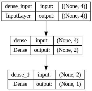
No wonder - the model is simple, with just three layers, including input and output.
# Import keras
from tensorflow import keras

# Plot the model with keras utils
from keras.utils import plot_model

# See the inputs and outputs of each layer
plot_model(model, show_shapes=True)
Please consider improving this network’s performance as the second task in your homework. Did you get better accuracy? Please let me know. I am curious!
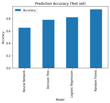
Comparing Performance
Prediction accuracy is a measure of how well a machine learning model is able to predict the correct target values for new, unseen data. It is expressed as a percentage and is calculated by dividing the number of accurate predictions made by the model by the total number of predictions. The prediction accuracy can be used to evaluate the performance of a model and compare it with other models.
The four models, trained on the same Sex, Pclass, Age, and Fare features and evaluated on the same held-out test set, produced the following test accuracies:
| Model | Library | Test accuracy |
|---|---|---|
| Random Forest | scikit-learn | 0.95 |
| Logistic Regression | scikit-learn | 0.82 |
| Decision Tree | scikit-learn | 0.78 |
| Neural Network | TensorFlow / Keras | 0.65 |
Let’s draw the bar plot of test accuracies for the evaluated models. The Random Forest is the best!
import matplotlib.pyplot as plt

accuracy_results_df = pd.DataFrame([{"Model": "Neural Network", "Accuracy": 0.65},
                                    {"Model": "Decision Tree", "Accuracy": 0.78},
                                    {"Model": "Logistic Regression", "Accuracy": 0.82},
                                    {"Model": "Random Forest", "Accuracy": 0.95}])


# Create a bar plot of the accuracy results
accuracy_results_df.set_index(["Model"]).plot.bar()

# Add a title and labels to the plot
plt.title('Prediction Accuracy (Test set)')
plt.xlabel('Model')
plt.ylabel('Accuracy')

# Show the plot
plt.show()
Conclusion
In this post, we created and evaluated several machine-learning models using the Titanic Dataset and predicting passenger survival. We have compared the performance of the Logistic Regression, Decision Tree and Random Forest from Python’s library scikit-learn and a Neural Network created with TensorFlow. The Random Forest Performed the best!
Random Forest is an ensemble classifier that aggregates many decision trees to reduce variance and overfitting; on this Titanic test set it reached 0.95 accuracy, outperforming Logistic Regression (0.82), the single Decision Tree (0.78), and the shallow Neural Network (0.65). For small, mostly tabular datasets like Titanic, tree-based ensembles typically beat an untuned, unscaled neural network.
In my next posts, I will show how we can do Cross Validation and model tuning, which are essential parts of ML experimentation. I will also give some examples of model overfitting. Please keep reading and subscribe to be in time for my next posts!
Frequently Asked Questions: Machine Learning on the Titanic Dataset
Why did Random Forest outperform the Neural Network on the Titanic dataset?
Random Forest is an ensemble of decision trees that captures non-linear feature interactions with no feature scaling and minimal tuning, reaching 0.95 accuracy on this Titanic test set. The shallow two-layer Neural Network (0.65 accuracy) was undertrained: only 10 epochs, unscaled inputs, and a 2-neuron hidden layer. Scaling features with StandardScaler and training for more epochs typically closes most of that gap.
How do I handle missing values in the Titanic dataset with Pandas?
The Titanic Age column has 177 missing values and Cabin has 687. Use df['Age'].fillna(df['Age'].median()) for numeric columns and df['Embarked'].fillna(df['Embarked'].mode()[0]) for categorical ones. In pandas 2.x, calling df.fillna(df.mean()) on a frame that still contains string columns raises TypeError: could not convert string to float, so select numeric columns first with df.select_dtypes(include='number').
Which features best predict Titanic passenger survival?
Sex is the strongest single predictor, followed by Pclass (passenger class) and Fare. The Decision Tree’s feature_importances_ attribute places Sex at the root split. Age adds predictive value for children. Models that combine Sex, Pclass, Age, and Fare reach roughly 80–95% accuracy on the test set.
Should I use accuracy or F1-score to evaluate a classification model?
Use accuracy when classes are roughly balanced, as in the Titanic survival task. When classes are imbalanced, prefer precision, recall, or the F1-score (the harmonic mean of precision and recall), because a model can post high accuracy simply by predicting the majority class every time.
Did you like this post? Please let me know if you have any comments or suggestions.
Posts about Machine Learning that might be interesting for youDisclaimer: I have used chatGPT while preparing this post. This is why I have listed the chatGPT in my references section. However, most of the text is rewritten by me, as a human, and spell-checked with Grammarly. All code snippets were tested in the Google Colab, and the Jupyter notebook is in my GitHub repository. Thanks for reading!
References
2. New Chat (chatGPT by OpenAI)
3. Feature importances with a forest of trees
4. Sklearn.ensemble.RandomForestClassifier
5. sklearn.linear_model.LogisticRegression
6. Data exploration and analysis with Python Pandas
8. Pandas Installation, TensorFlow and Sckikit-learn
11. Partial Dependence and Individual Conditional Expectation plots
Enjoyed this? Get more like it.
Weekly notes on AI tools, Python, and what I'm actually building — plus a free copy of Fantastic AI: The 2026 Toolkit.